Channel Calibration Demonstration
In the course of this example, we will:
| • | Demonstrate the effect of channel calibration on the data display. |
We will now proceed to open a new histogram to show how the calibration affects how the data is displayed.
| 1. | Insert a new histogram using the file Monocytes.002 in the Tutorial Sample Data archive. |
| 2. | Set the new histogram to display channel FL3-H. |
| 3. | Make sure the histogram is ungated. |
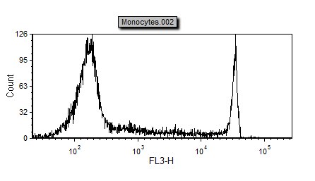
The histogram should look similar to Figure T23.9. Note that the x-axis extends from less than 102 to more than 105. The axis is shown as calibrated, expressing the mean equivalent number of soluble PE-Cy5 molecules. This is because the default setting for all plots is to use calibrated axes.

Figure T23.9 Histogram with Calibrated Axis
| 4. | Right-click on the histogram to bring up the associated pop-up menu. |
| 5. | Select Histogram Statistics from the pop-up menu. |
The Statistics window associated with the histogram will appear.
| 6. | Move the Statistics window under the histogram. |
| 7. | Click inside the Statistics window so that it is selected; it should have a green border. |
| 8. | Select the Format→Statistics Options→Statistics command (Figure T23.10). |

Figure T23.10 Selecting the Format Statistics Command
The Formatting Statistics dialog now appears.
| 9. | Select the following items on the Formatting Statistics dialog: Median, Geometric Mean, Arithmetic Mean, CV. |
| 10. | Deselect all other items from the Formatting Statistics dialog. |
| 11. | Click OK. |
The Statistics window should appear similar to Figure T23.11.

Figure T23.11 Statistics Window for Histogram with Calibrated Axis
| 12. | Right-click on the histogram to bring up the associated pop-up menu. |
| 13. | Select Format from the pop-up menu. |
The Formatting dialog now appears.
| 14. | Move the Formatting dialog so that both the histogram and the statistics window are visible. |
| 15. | Select Histogram→Histogram Specific Options from the categories listed on the left of the Formatting dialog, as previously shown in Figure T23.4. |
Notice that the Use channel calibration on axis is checked.
| 16. | Deselect the Use channel calibration on axis option (Figure T23.4). |
| 17. | Click the Preview button. |
Note that the histogram curve itself does not change, but the axis reverts to the usual 100 to 104 uncalibrated scale. Notice that the values in the statistics window change when the axis changes from calibrated to uncalibrated. When calibration is active, the units represent the MESF of PE-Cy5. When calibration is not used the units are the arbitrary values obtained from the raw data in the FCS file.
| 18. | Click Cancel to close the Formatting dialog. |
In the next section, we will cover saving and loading channel calibrations.
