Importing Single Image Data
This section pertains to data from a set of single images that were not obtained from a 96 well plate, such as images obtained from a slide.
After adjusting the export settings in CellProfiler and running your pipeline, you may proceed to analyze your images and import the data into FCS Express V5.
| 1. | Load the Section2pipelineCOMPLETED.cp pipeline in CellProfiler. |
| 2. | Select the default input and output folders in CellProfiler to load and store the data as in Figure T24.13. |
| 3. | Analyze the images in CellProfiler. |
Importing the Single Image Experiment to FCS Express
Note on FCS Express Preferences before starting these steps of the tutorial:
The File selection dialog must be enabled:
| A. | Open the FCS Express User Options by choosing File→Options. |
| B. | Flag the "When creating a new plot, always display the selection dialog" box in the Files/Directories category. |
(Enabling this feature is not a requirement of FCS Express, it has been selected for convenience in this tutorial)
| 4. | Open FCS Express V5. |
| 5. | Open the FCS Express User Options by choosing File→Options |
| 6. | Select Cell Profiler Options from the Data Loading category (Figure T24.19). |
| 7. | Select csv from the delimiter drop-down list. |
| 8. | Check the Load Images check box. |
| 9. | Uncheck the Load path names from Cell Profiler table of contents file check box. |
| 10. | Click OK to close the FCS Express User Options dialog. |
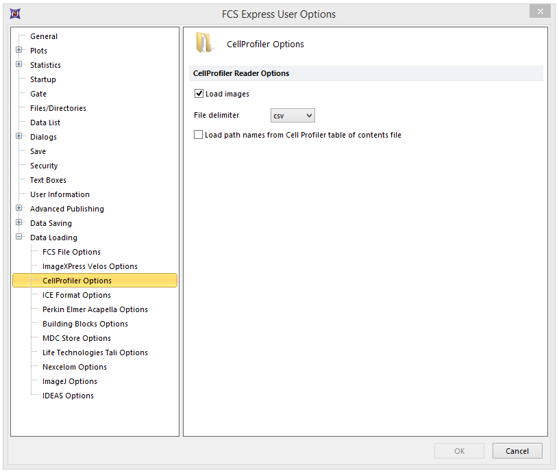
Figure T24.19 CellProfiler Data Loading Options
| 11. | Select the Insert→2D Plots →Picture Plots command (Figure T24.20). |

Figure T24.20 Choosing a Picture Plot to Insert
| 11. | Click anywhere on the layout and the Select a Data File dialog will appear. |
| 12. | Browse to the Default Output Folder where you stored your output data from CellProfiler. |
| 13. | Change the Files of type: drop-down list to CellProfiler (*.cpout) (Figure T24.21). Icons for the documents outputted by CellProfiler will appear. For this example, they will be labeled cells_05.cpout and nuclei_05.cpout. |
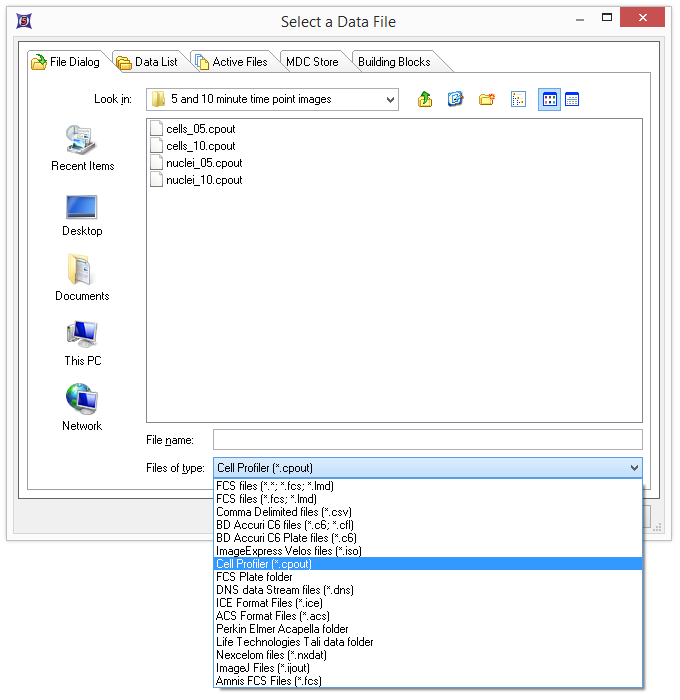
Figure T24.21 Select a Data File Dialog
| 14. | Highlight cells_05.cpout and click Open. |
Note: For this example, we will use cells_05.cpout which will display data from the 5 minute time point objects classified in the IdentifySecondaryObjects module of CellProfiler which corresponds to the entire cell area. Nuclei_05.cpout will display data from the 5 minute time point objects classified in the IdentifyPrimaryObjects module of CellProfiler which corresponds only to the nuclear area of the cells.
| 15. | Highlight Cytoplasm from the Image Parameter list box of the Open 2D Plots dialog (Figure T24.22) to view the cytoplasmic image. |
| 16. | Click OK. |
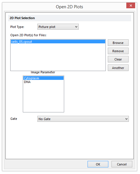
Figure T24.22 Choosing Image Parameters from the Open 2D Plots Dialog
A Picture Plot will now appear on your layout indicating that the data was successfully imported (Figure T24.23).
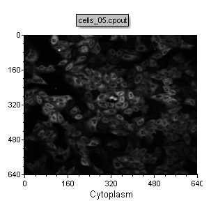
Figure T24.23 Example of the Cells (5 Minute Time Point) Picture Plot
| 17. | Repeat steps 11-16 but highlight DNA as Image Parameter in the Open 2D Plots dialog. |
Note: alternatively to step 17 you can duplicate 2D plot previously created and then change the visualized parameter by clicking on the X axis and choosing DNA instead of Cytoplasm.
The layout should now looks like Figure T24.23b.
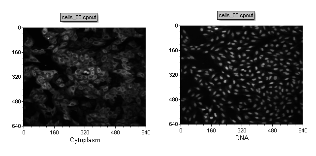
Figure T24.23b Picture plots of the cells_05.cpout file depicting cytoplasm and DNA
| 18. | Any type of 2D plot can be created by following the previous step. For training purpose, the user can try opening two Color Dot Plots of the same file (i.e. cell_05.cpout) depicting: |
- AreaShape_Area with Intensity_MeanIntensity_Cytoplasm
- AreaShape_Area with Intensity_MeanIntensity_DNA
The layout should now looks like Figure T24.23c.
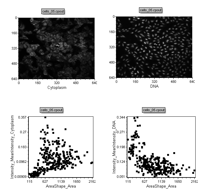
Figure T24.23c Picture plots and Scatter plots of the cell_05.cpout file
Any 2D gate can easily be created on the Picture Plots and on the Scatter Plots as well. Inserting a new 2D plot gated on the picture plot gate will allow you to view the data as familiar dot plots, or view gated portions of the image (Figure T24.24).
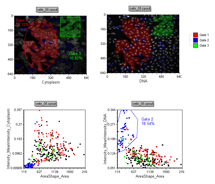
Figure T24.24 Example of Gating on a Picture Plot and Backgating from a Dot Plot to a Picture Plot
In the next exercise, we will export numeric data only from a 96 well plate.
