Using Parameter Math
It is often useful to define a ratio when examining kinetics data. This can be a ratio of two different dyes, or the ratio of the same dye in two different emission wavelengths. The parameter math feature of FCS Express allows the user to define mathematical operations from simple ratios to complex formulas for use in your analysis. FCS Express will also calculate and display the actual ratio values rather than an arbitrarily scaled multiplied integer as some other software packages do.
In this section you will learn how to create parameter math formulas for use in Kinetics Plots.
Although any kinetics data files of your own can be used to follow along in this tutorial, you have the option of using the same sample data files used in this tutorial. The sample data files are located in the Tutorial Sample Data archive. The KineticsTutorial.fey, kinetics10.010, and kinetics25.025 data files have been embedded and will be used here.
1.Select File tab→Open Layout.
2.Select the KineticsTutorial.fey layout file located in the FCS Express Sample Data directory from the Load Layout dialog.
In the KineticsTutorial. fey layout the two samples (kinetics10.010, and kinetics25.025) are already displayed as kinetics plot.
The following steps open the transformation window and create a new Parameter Math transformation:
3.Open the Transformation window by selecting the Tools tab→Transformations →Transformations command ![]() (Figure T21.1).
(Figure T21.1).
4.Click on the drop down arrow adjacent to the blue plus ![]() button
button ![]() in the transformations dialog(Figure T21.1).
in the transformations dialog(Figure T21.1).
5.Click on Parameter Math in the drop down list ![]() (Figure T21.1).
(Figure T21.1).
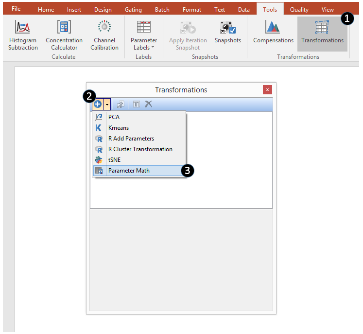
Figure T21.1 Selecting the Parameter Math transformation.
A New Parameter Math transformation is created and listed in the upper part of the Transformation Window. The Parameter Math dialog now appears in the lower part of the Transformation window as seen in Figure T21.2. Note that the kinetics10.010 sample has been automatically selected as template file in this example but this can be changed by clicking on the ellipsis ![]() at the right of the Template File field.
at the right of the Template File field.
6.Choose New in the Parameter Math dialog (Figure T21.2) to define a new formula.
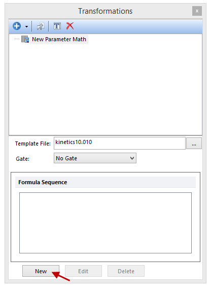
T21.2 The New Parameter Math dialog as it appear in the Transformation window after Step 5.
A Create New Sequence Item window similar to the one represented in Figure T 21.3 will open.
The following instructions refer to Figure T21.3.
5.Enter Ca++ Ratio in the Output Parameter Name box ![]() .
.
6.Change the First Input Parameter to Fluo 3 ![]() .
.
7.Change the mathematics operator to "/" for division ![]() .
.
8.Change the Second Input Parameter to Fura Red ![]() .
.
9.Click OK ![]() .
.
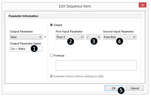
Figure T21.3 Defining a Parameter Math Sequence Item Formula
The Parameter Math dialog in the Transformation window now displays the formula sequence we defined (Figure T21.4). Please note that, although in this example the New Parameter Math transformation contain only the Ca++ Ratio formula, a Parameter Math transformation can contain more than one formula.
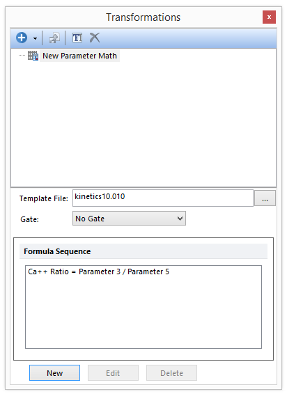
Figure T21.4 Parameter Math Sequence Dialog with Formula Displayed
The Parameter Math transformation has now been defined and can now be applied to plots for display and analysis.
We will now apply the New Parameter Math transformation (containing the Ca++ Ratio formula) to the histograms displayed in the layout.
Please note that the New Parameter Math transformation has been created using the kinetics25.025 sample as Template File. Though, since the kinetics10.010 sample has the exact same parameter in the same exact order, we can apply the New Parameter Math transformation to this sample as well.
10. Left click and hold on the New Parameter Math transformation from the Transformation window.
11. Drag the New Parameter Math transformation out of the Transformation window and release it on top of each of the 1D plot (Figure T21.5).
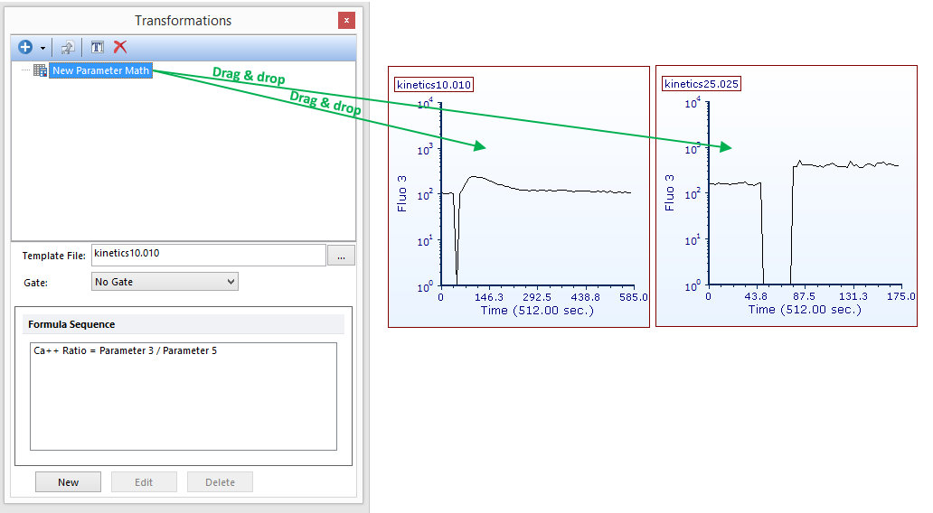
Figure T21.5. Use Darg&Drop to apply the Parameter Math transformation to the plots of the layout.
The two 1D plots should now look as the ones displayed in figure T21.5b. Note the suffix Parameter Math applied automatically added to the plot title.
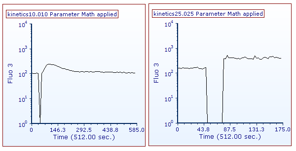
Figure T21.5b The two kinetics plot as they appear when the New Parameter Math transformation has been applied to them.
The newly calculated Ca++ Ratio parameter can now be accessed as a standard parameter from the axis labels.
We will now display the Ca++ Ratio parameter on the Y axis of both 1D plot simultaneously via the formatting windows.
12.Hit Ctrl+A to select all plots.
13. Choose the Format → Plot Option → Overlay command from the Ribbon.
14. Change the Y Parameter to Ca++ Ratio (i.e. the formula defined in the New Parameter Math transformation) from the drop-down list (Figure T21.6)
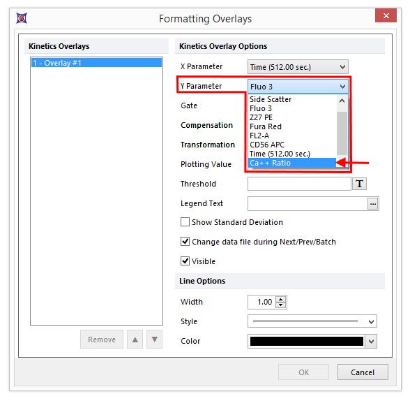
Figure T21.6 Changing the Y Axis to the Ratio Defined by the Parameter Math
The plots on the layout should now look like Figure 21.7. Since the first parameter of the parameter math calculation was a logarithmic parameter, FCS Express assumed the newly created parameter should be a log parameter as well. This is typically the case, but in this situation it is not correct. Since the plots display the real ratio value, we will have to adjust the axis settings to display the data on a linear scale.
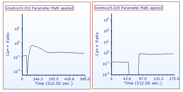
Figure T21.7 Ca++ Ratio vs Time
15. Hit Ctrl+A to select all plots.
16. Choose the Format→Plot Options→Axes command from the Ribbon.
Refer to Figure T21.8 for the following steps.
17. Under the Select Axis section, select Y-Axis ![]() .
.
18. Under the Scale section, un-check Automatic ![]() .
.
19. Change the Scale to Linear ![]() .
.
20. Under the Range section, un-check Automatic ![]() .
.
21. For Minimum, enter 0 ![]() .
.
22. For Maximum, enter 1 ![]() .
.
23. Click OK ![]() .
.
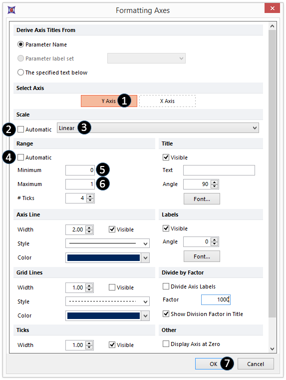
Figure T21.8 Formatting Axes Dialog
The plots in the layout should now look like Figure T21.9.
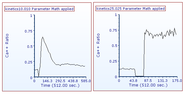
Figure T21.9 Plots Scaled Correctly to Display the Ca++ Ratio
In the next section, we will apply gating and statistics to kinetics plots.
