In the course of this example, we will:

•Identify the variables needed for calibrating the channels.

•Set up the Channel Calibration tool using the beads and markers prepared in the previous section.

•Obtain the calibration information.

 

Before we can begin our setup, it is important to clarify a detail on how flow cytometry FCS data files are formatted. Typically, in an FCS file, the first parameter described is Forward scatter, followed by Side scatter, and then the fluorescent channels in order – FL1, FL2, FL3, etc. Some instruments embed the name of the parameter directly in the FCS file and you can see it in the Channel Calibration tool (see instructions below). In the file we will be using for this tutorial, that is not the case. Nevertheless, we know that "Parameter 5" corresponds to FL3, which is the channel we want to calibrate. In case you do not know which parameter corresponds to a fluorescent channel, you can view the FCS text header information by selecting the Data→DataInfo→View Header command.  A dialog displaying the FCS data file header information will appear displaying all the parameter information in a grid.

 

We will now proceed to set up the Channel Calibration tool.

1.Select the Tools→Calculate →Channel Calibration command (Figure T23.5).

 

 

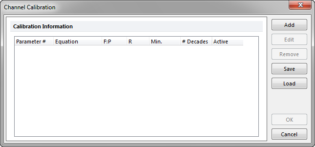
The Channel Calibration dialog appears (Figure T23.6).

 

 

2.Click the Add button on the Channel Calibration dialog (Figure T23.6).

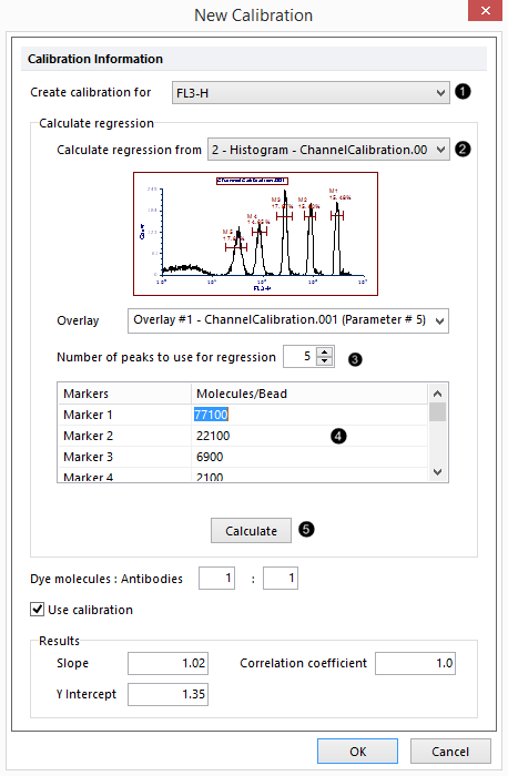
A New Calibration dialog now appears, similar to Figure T23.7.

 

 

3.Select FL3-H from the Create calibration for drop-down list (Figure T23.7).

4.Select the Histogram - ChannelCalibation.001 (FL3) with the calibration beads from the Calculate regression from drop-down list.

Note: If there are multiple overlays in your histogram, you can select which one to use in the Overlay option. In this case it is a simple histogram. Therefore, there are no other overlays and nothing has to be changed.

5.Enter "5" in the Number of peaks to use for regression field.

Usually, it is best to use all available peaks (except the blank one); but if for some reason you want to omit one of the peaks, you can do so. You must use a minimum of three peaks to calculate a regression.

6.Enter the following fluorescence values, shown in Figure T23.7, for each peak, in the Molecules/Bead column beginning with Marker 1; 77100, 22100, 6900, 2100, 750.

These values are provided by the manufacturer of the beads, usually quoted as MESF – Mean Equivalent of Soluble Fluorochrome. In this case, the reported MESF are for PE-Cy5 molecules.

If you specified fewer peaks than the number of markers in the histogram, for example, four peaks out of five markers, make sure you select the correct markers in the left column.

7.Click the Calculate button (Figure 7).

The New Calibration dialog and results, i.e., Slope , Y intercept , and Correlation coefficient , should look similar to Figure T23.7. FCS Express calculates the regression using the logarithmic values. The minimal detection threshold is the fluorescence obtained by setting the channel to "1" in the regression equation. The number of decades (the dynamic range of the machine) is calculated as the inverse of the slope.

8.Click OK to close the New Calibration dialog.

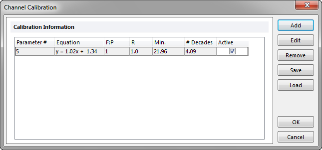
The Channel Calibration dialog will now appear similar to Figure T23.8. The channel calibration is now ready for use.

As you define calibrations for more than one parameter, they will all appear here. If the Active option is set, then that calibration set will be used in the layout (in those plots that have the Use channel calibration on axis checked. You can only have one active calibration defined for a particular parameter.

 

 

Note: Although we won’t show it in the tutorial, you can also edit existing calibrations for a particular parameter by selecting the parameter in the Channel Calibration list and pressing the Edit button.

9.Click OK to close the Channel Calibration dialog and return to the layout.

 

Next, we will demonstrate channel calibration.