•Create Conditional Formatting using custom tokens.

•Insert Conditional Formatting into the new Spreadsheet.

 

Using the 'BShift' and Custom Token data created in the last section, we will now define conditional formatting ('NEG', 'POS', and 'WEAK') in the Spreadsheet. We will use conditional formatting to classify our samples and ultimately determine the status of the patient serum cross-match. To begin, we will insert a new Spreadsheet.

 

1.Open the HLA Conditional Formatting.fey found in the FCS Express Sample Data folder.

We will now begin defining Conditional Formatting to classify the results for each sample in the spreadsheet.

2. Click on the Page 3 tab.  

3.Click on the header of the 'B' column on the spreadsheet.

4. Click on the Spreadsheet Tab→Layout Tab→Formatting and Sorting→Conditional Formatting.

5. Mouse over Icon Sets.

6. Mouse to the right to reveal the available icon set.

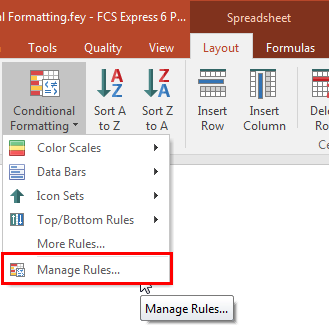
7. Left Click the first set of arrows icons in the first row, shown by the red box as in Figure T15.40 below.

 

 

You will notice that the data set has now been conditionally formatted based to use the icon set based on the default rules. We will now adjust the rules to perform a custom classification using the icon sets.

6. Click on the Spreadsheet Tab→Layout Tab→Formatting and Sorting→Conditional Formatting.

7. Click on the drop down menu to Managing Rules (as seen enclosed in the red box in Figure T15.41).

Note: Here we will define the rules for the conditional formatting seen in Figure T15.41. Before using the Manage Rules feature make sure the column containing the data set to classify in the spreadsheet is selected. For example; in this tutorial, it will be column 'B'.

 

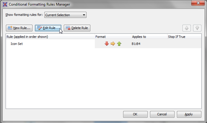
8. Click on the words Icon Set underneath the Rule column in Figure T15.42

9. Click on the Edit Rule... button (shown with the cursor on it in Figure T15.42).

Note: During conditional formatting, we can also add additional rules. In this particular case, we will edit the rule as it is already started in this particular layout (shown by the cursor). This rule will apply to cells B1-B4 as is shown in Figure T15.42.

 

 

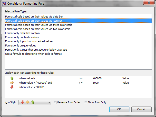
10. Click on Format all cells based on their values via icon set as in Figure T15.43 (shown highlighted in blue).

Note: Here you will add values according to each rule displayed by the icon set. Make sure you choose the rule type. In this tutorial, we are using Format all cells based on their values via icon set.

 

 

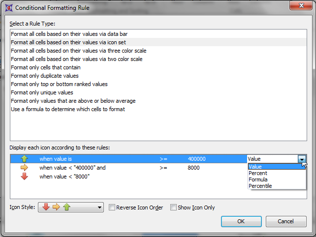
11. Click on the percent drop down in the Up Arrow category Figure T15.45.

12. Choose value as in Figure T15.45.

13. Click on the "0" in order to enter a new value.

14. Enter the value of 40000 to replace "0".

Note: In this case, we entered 40000 which defines greater than or ">" 40000 for the green arrow.

 

In order to define the second line for the right facing yellow arrow in the Display each icon according to these rules: window;

15. Click on percent in the second row.

16. Choose value from the drop down.

17. Click on the "0" from the second line in the Display each icon according to these rules: window.

18. Enter 8000 as the numerical value for the yellow arrow.

Note: The yellow rule is defined by less than or "<" 40000 but greater than of ">" 8000.

Also Note: The red arrow is then automatically defined as less than or "<" 8000.

19. Click OK. The formatting rules dialog will appear as in Figure T15.45.

20. Click Apply.

21. Click OK.

 

Note: you will see the conditional formatting defined in the spreadsheet shown in Figure T15.46. To see the changes in real-time you may type in a different value in column B or update the Lymphs gate on Page 1 or Page 2. The conditional formatting will change due to the values in the cells updating.