Automatic Compensation and Batch Processing
In FCS Express, you may define a post-acquisition compensation matrix using single-stained controls, apply it to your experimental samples, and batch process your results to Microsoft PowerPoint, PDF, and Word, all within a single layout. There is no need to export and import compensation into separate layouts.
In this section, we will:
•Change our default options to use a post-acquisition compensation matrix as default
•Set an automatic compensation as default for the entire layout
•Insert plots of experimental files in the same layout
•Batch process the results to Microsoft Office PowerPoint
We will begin with a layout in which an automatic compensation was already defined, using single-stained controls.
1.Select File tab→Open.
2.Open the layout AutoCompWithBatchProcess.fey from the Tutorial Sample Data archive.
NOTE: An automatic compensation already has been defined in this layout, according to Steps 1-27 of this section of this tutorial. We will set this compensation as default for the entire layout.
3.Select File tab→Options.
4.If necessary, select Compensation Default, then FCS File from the Default Compensation to Use drop-down list and click OK (Figure T8.33). Learn more about Compensation Default Options.
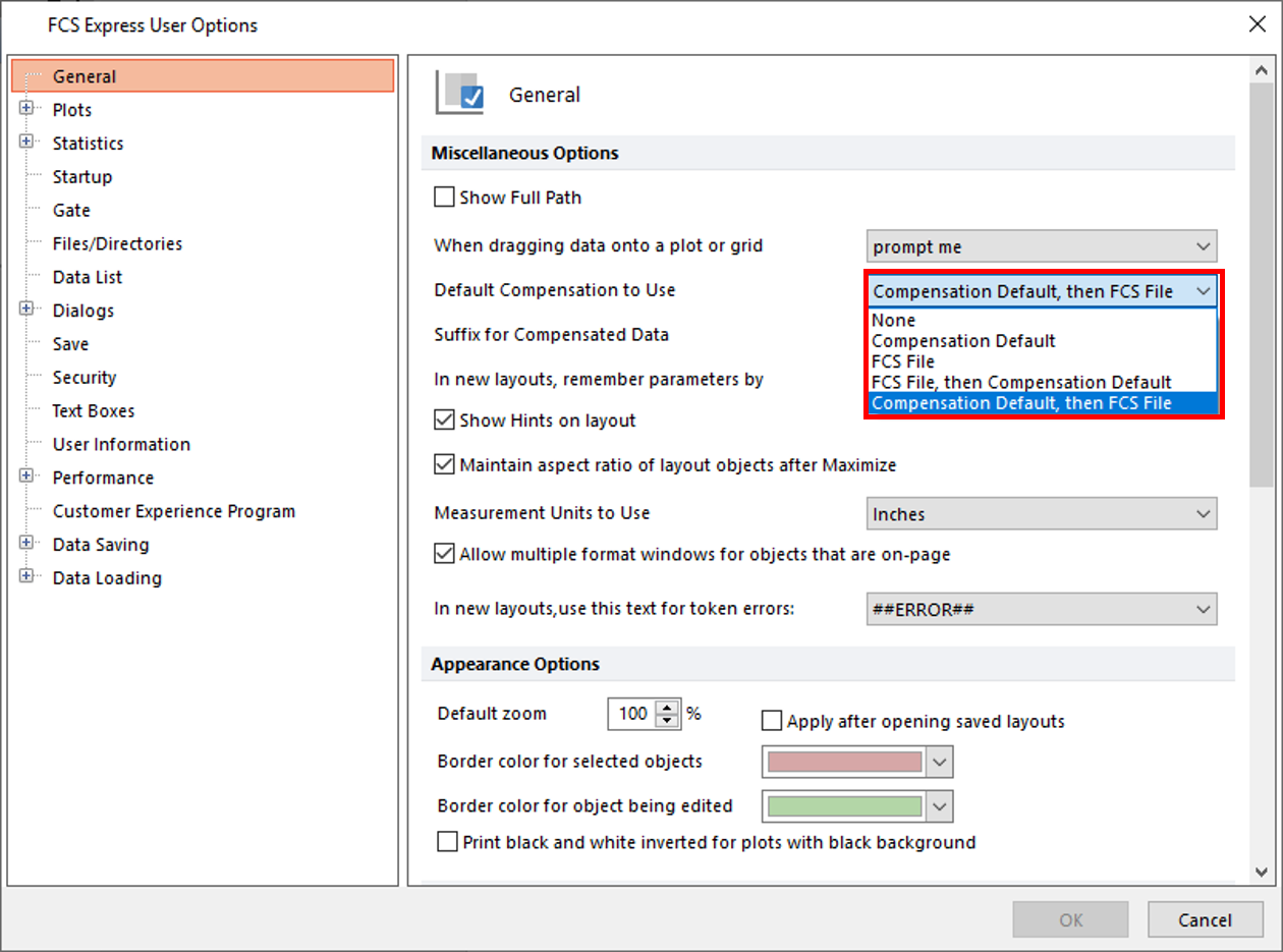
Figure T8.33 Changing the Default User Option for Compensation
5.Click to expand the Created manually node within the Compensations window (Figure T8.34, ![]() ).
).
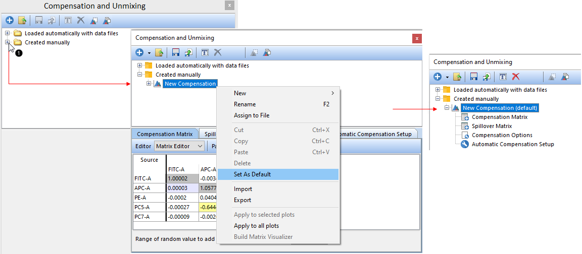
Figure T8.34 Setting a compensation matrix as default for the layout
6.Right-click on the New Compensation name and choose Set As Default (Figure T8.34, ![]() ). This matrix will now be marked as default (Figure T8.34, right).
). This matrix will now be marked as default (Figure T8.34, right).
We will now insert plots of experimental files in the same layout, and watch as the Compensation Default matrix is automatically applied.
7.Drag the first file from the Data List to an empty spot on the layout (Figure T8.35, ![]() ).
).
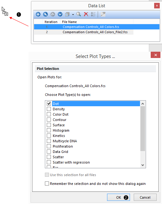
Figure T8.35 Inserting a plot on the layout
8.Click OK (Figure T8.35, ![]() ).
).
9.Click and change the X- and Y-axis labels to change the parameters displayed on the newly-inserted plot to "CD95 PC5-A" (Figure T8.36, ![]() ) and "CD8a PC7-A" (Figure T8.36,
) and "CD8a PC7-A" (Figure T8.36, ![]() ), respectively.
), respectively.
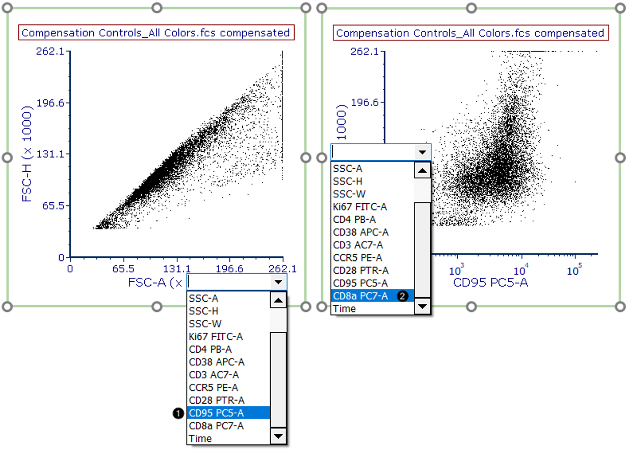
Figure T8.36 Changing axis parameters
The Compensation Default matrix has been applied automatically to the plot. You may verify this is true in the following ways:
•Manually changing the values in the Compensation Matrix from the Compensations window and watching the events update (Figure T8.37, cell in matrix for PC5-A vs PC7-A)
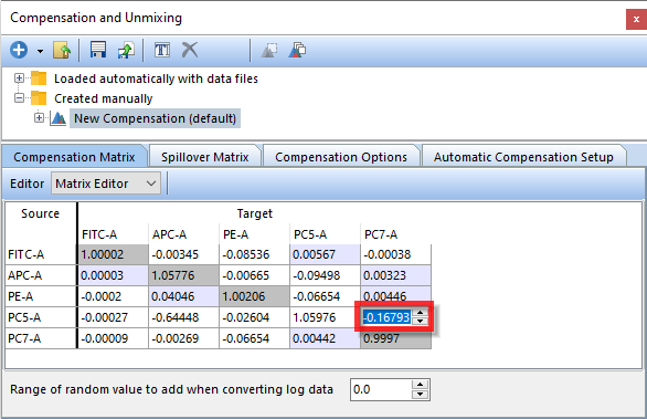
Figure T8.37 Editing a compensation matrix manually
•Right-clicking the plot to see the name of the compensation applied (Figure T8.38)
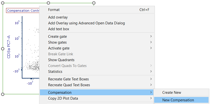
Figure T8.38 Compensation Name Applied to Plot
•Double-clicking the plot or right-clicking it and choosing Format to view the Compensation in the Overlays category of Formatting dialog (Figure T8.39)
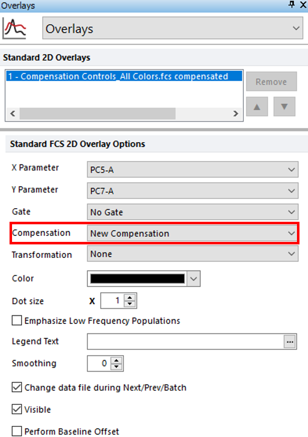
Figure T8.39 Compensation Information from Formatting dialog
We now will perform a Batch Process to export the results from all the files in our Data List to PowerPoint. The Batch Process Action has already been set up for convenience. To learn more about this functionality, see the Batch Processing tutorial or the short Batch Processing video on YouTube.
10. Click Batch & Export tab→Batch Export to PDF, PowerPoint, Excel, Prism, ... group→Run command ![]() .
.
A PowerPoint file with the results from all the files in your Data List has now been saved on your Desktop. If the PPT file does not open automatically, please change the Export to PowerPoint's Output file options save path to a valid one for your computer. See the PowerPoint section of the Batch Processing tutorial for details.
