Analysis of 3 Cycle Data
Analysis of DNA histogram containing multiple cycling populations requires the advanced Multicycle version, which must be purchased separately. We will begin by opening a new blank layout page and inserting a Multicycle DNA plot to view multiple cycles within the data.
1.Select File tab→New→New.
2.Select the Insert tab→1D and 2D Plots group→Fit→Multicycle DNA command.
3.Click on a white, blank area of the layout.
The Select data file dialog appears, previously shown in Figure T21.1.
4.Navigate to the Tutorial Sample Data directory.
5.Select the file ASCII4.fcs.
6.Click Open.
The Multicycle DNA plot now appears (Figure T21.30). Note the two aneuploid populations, shown in blue and green, comprise the majority of this histogram.
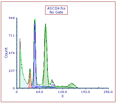
Figure T21.30 MultiCycle DNA Histogram with Two Aneuploid Populations
You could insert the DNA Cycle, DNA Model Summary, and DNA Experiment Statistics windows as previously shown to further study this histogram. However, it is apparent that this DNA histogram has multiple cycling populations, which MultiCycle appears to have identified correctly.
We now will look at a histogram that is more difficult to analyze. Due to the aneuploid populations overlapping, the Autofit function of MultiCycle does not correctly identify the two aneuploid populations, requiring us to use manual settings. We will begin by inserting a histogram.
7.Select the Insert tab→1D Plots→Histogram command.
8.Click on a blank area of the layout.
A histogram of the current data file appears on the layout. We will now change the data in the plot.
9.Right-click the histogram and select Change file.
10. Select the file ASCII8.fcs from the Select a Data File dialog which appears.
11. Click Open.
12. Right-click on the histogram and select Format and choose Overlays from the dropdown menu to adjust the Smoothing (Figure T21.31).
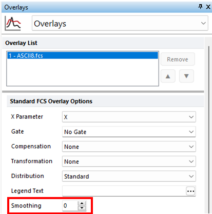
Figure T21.31 Modifying Smoothing on Histogram
The histogram changes to display the ASCII8.fcs data file (Figure T21.31). Note there is an aneuploid peak (Figure T21.32, red circle). However, upon closer examination, it appears there may be two aneuploid peaks with very similar amounts of DNA. If not well observed expand the width of the histogram plot. We will use the Autofit function of MultiCycle to analyze this DNA histogram and show that it does not yield correct results in this case.
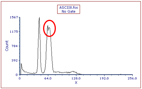
Figure T21.32 ASCII8.fcs Histogram
12. Select the Insert tab→1D and 2D Plots→Fit→MultiCycle DNA command (Figure T21.4).
13. Click on a blank area of the layout.
The Multicycle DNA plot now appears as shown in Figure T21.33. The Autofit function of MultiCycle has analyzed this histogram using a two cycle model, thereby assuming there is one aneuploid population, shown in blue. We will now use Multicycle to analyze the DNA histogram without using Autofit.
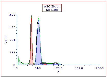
Figure T21.33 Autofit MultiCycle Analysis of ASCII8.fcs
14. Double-click the Multicycle plot. The Format dialog will appear, docked to the right.
15. Select the DNA Fit category.
16. Uncheck the box next to Detect fit type automatically (Figure T21.34, ![]() ). This turns off Autofit.
). This turns off Autofit.
17.Select 3 Cycle from the Fit Type drop-down list (Figure T21.34, ![]() ).
).
18. Check the box next to Diploid CV = Aneuploid CV (Figure T21.34, ![]() ).
).
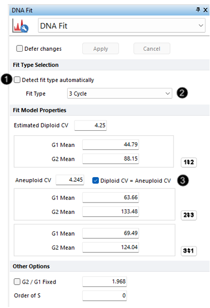
Figure T121.34 Formatting Fit Model Options
We have turned off Autofit and updated Multicycle to apply a 3 Cycle model. We also have specified the additional constraint on the model that the CV of the diploid peak should equal the CV of the aneuploid peaks. The Multicycle analysis using the manual fit options appears below (Figure T21.35).
Alternatively, you can turn off Autofit and specify a 3 Cycle model from the Multicycle tab:
•Click the Multicycle plot to select it.
•Click the Multicycle tab→Fit Parameters group→Autofit command to turn off Autofit.
•Click Multicycle tab→Fit Parameters group→3 Cycle option from the Cycle drop-down list.
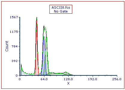
Figure T21.35 Manual MultiCycle Fit
