Conditional Formatting
Conditional formatting is a tool that allows you to apply different displays in the form of Color Scales, Data Bars, and Icon sets to a range of cell values. Conditional formatting may be applied by:
1. Select a range of cells in a Spreadsheet.
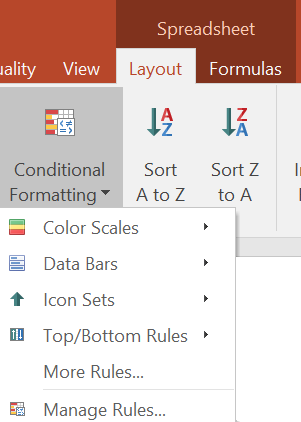
2. Click on the Spreadsheet tab→Layout tab→Formatting and Sorting→Conditional Formatting dropdown (Figure 11.11).

Figure 11.11 - Choosing conditional formatting from the Spreadsheets--> Layout tab.
3. Choose the type of display from Color Scales, Data Bars, and Icon Sets.
4. Choose the sub-type of conditional formatting you wish to apply.
The conditional formatting you choose will be applied to the range of cells. Below is an example of some conditional formatting options applied to a range of data Figure 11.12.

Figure 11.12 - A variety of conditional formatting options applied to a series of data.
The conditional formatting is based on a series of rules which may be managed by clicking on the Spreadsheet tab→Layout tab→Formatting and Sorting→Conditional Formatting dropdown→Manage Rules command. From within the Conditional Formatting Rules Manager you may select Edit Rule to adjust how color scales, bars, and icon sets values are determined.
