Automatic Compensation
To create a Compensation Definition automatically from single stained controls:
1.Select File tab→Open (Figure T3.1).
2.Open the layout AutoComp.fey found in the Tutorial Sample Data archive.
This is the layout that we are going to use to illustrate how to set up automatic compensation (Figure T8.6). Typically you would start with a blank layout but we have inserted plots so you can more easily see your data for the purposes of this tutorial. The top-left most plot is of FSC vs. SSC data with a gate based on a bead population. In order to use the automatic compensation, you need a single-stained control for every parameter that you wish to compensate as well as an unstained sample.
(Note: The unstained control can be a universal negative, a negative population defined by a gate, or the negative population with the tube of the positive control. In this case we will use an unstained sample)
The following data set contains an Unstained Control, All Color Control, and five single stain controls for the following parameters: FITC, PE, PC5 (PE Cy5), PC7 (PE Cy7), and APC. All of the histograms are gated on the Beads gate and display the data file and parameter for each control. For example, the top-right most histogram is the Compensation Controls_FITC Stained Control.fcs file and the FITC-A parameter is being displayed on the X-axis.
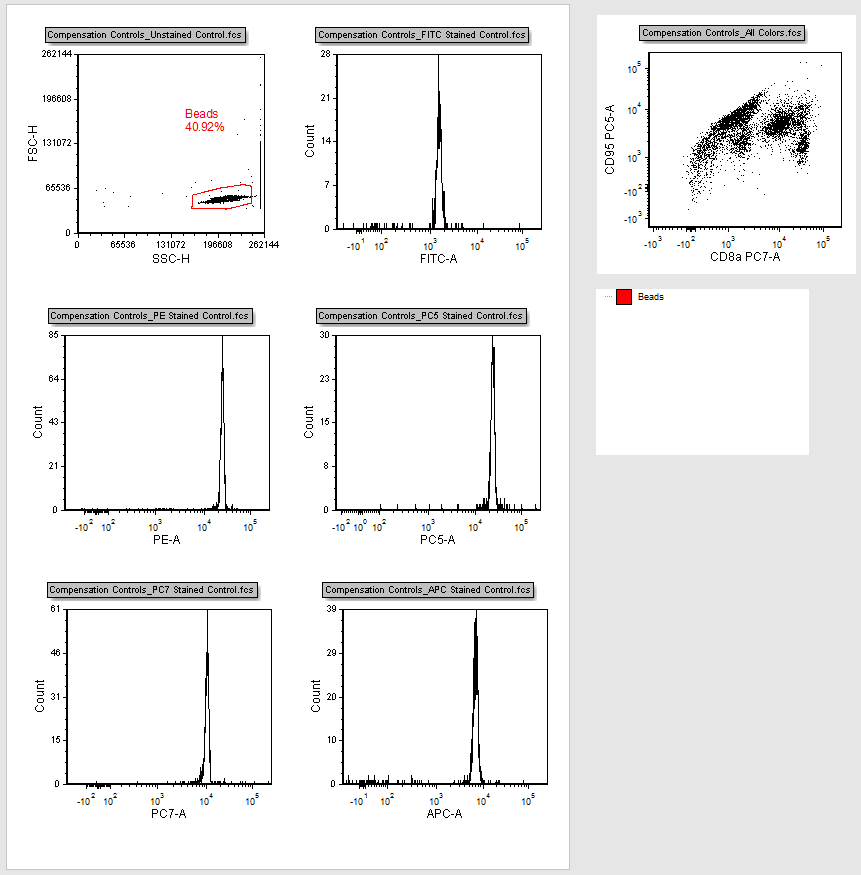
Figure T8.6 Autocomp.fey Layout
In this example, we are setting compensation for all five single stained controls/colors. However, you can set compensation for as many channels as you like, provided you have a single-stained control for each particular channel.
3.Click on the Tools tab→Transformations→Compensations command to open the Compensations navigator (Figure T8.7).
The Compensations navigator can be moved anywhere on the screen and it is dockable and pinnable. Please feel free to move it around the screen as needed while working on this tutorial.
4.Click on the blue plus button, ![]() , to Create a new compensation (Figure T8.7).
, to Create a new compensation (Figure T8.7).
A text box highlighted in blue will appear with the text New Compensation (Figure T8.7).
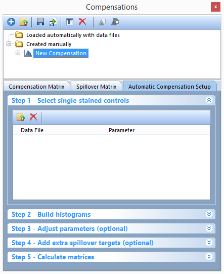
Figure T8.7 - The Compensations navigator. Use the navigator to add new compensations, edit definitions, and to create new Automatic Compensation Setups.
5.Click on the Add data for compensation button, ![]() , in the Automatic Compensation Setup→Step 1 - Select single-stained controls window (Figure T8.7).
, in the Automatic Compensation Setup→Step 1 - Select single-stained controls window (Figure T8.7).
6.The Standard Open Data Dialog will appear (Figure T8.8).
Note: based on your User Options, the Advanced Open Data Dialog may appear. If the Advanced Open Data dialog appears, please select the ![]() button to access the Standard Open Data Dialog.
button to access the Standard Open Data Dialog.
. Select FCS Files (*.*; *.fcs; *.lmd) from the files of type drop-down menu (Step 1, Figure T8.8).
.Select multiple files from your computer (Step 2, Figure T8.8).
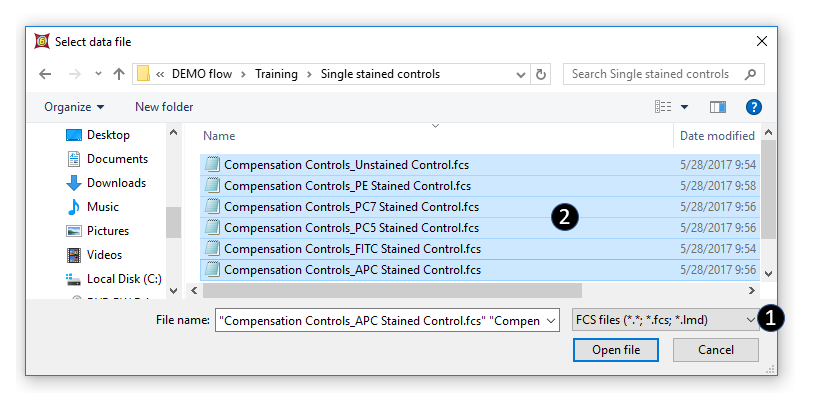
Figure T8.8 - Use the Select Data File window to select all of the files for use in the Automatic Compensation Setup.
7.Click Open file.
Notice that all of the single-stain control files and the unstained control file have been brought into the Select single-stain control window (Figure T8.9). We will now assign the correct parameter for each individual file by matching the single-stain control name in the file name to the Parameter in the -select parameter- drop down list.
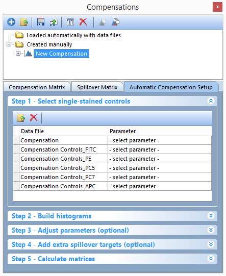
Figure T8.9 - Files have been added to Step 1 in the Automatic Compensation Setup. The Parameter column drop downs will be used to match the single stained sample data control files to the respective parameter for compensation.
8.Click on -select parameter- for the first file (Compensation Controls_Unstained Control.fcs) (Figure T8.10).
9. Select Universal Negative from the bottom of the -select parameter- drop down list (Figure T8.10).
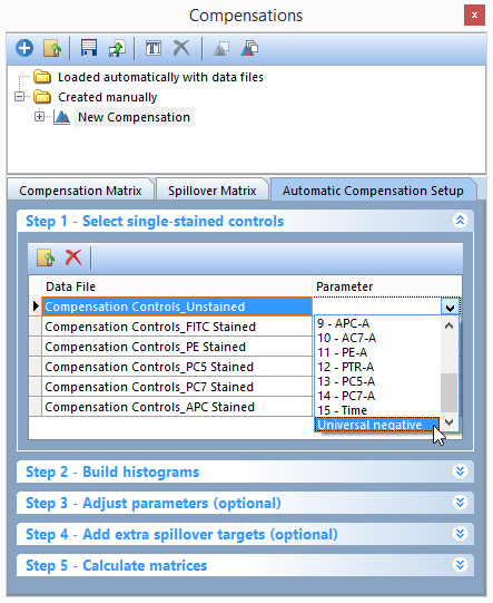
Figure T8.10 - Selecting the Universal negative parameter to match the Unstained Control.fcs file.
This will assign the Compensation Controls_Unstained Control.fcs file as the universal negative control for the rest of the single stained controls.
10. Click on -select parameter- for the second file (Compensation Controls_FITC Stained Control.fcs) (Figure T8.11).
11. Select 7- FITC-A from the -select parameter- drop down list (Figure T8.11).
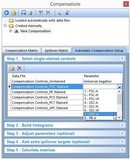
Figure T8.11 - Selecting the FITC-A parameter to match the FITC Stained Control.fcs file.
12. Repeat steps 11 and 12 for each of the single stained controls and parameters. For example, PE Stained Control.fcs should be matched with 11 -PE-A. The Step 1 - Select single-stained controls window should look like figure Figure T8.12 when you are done.
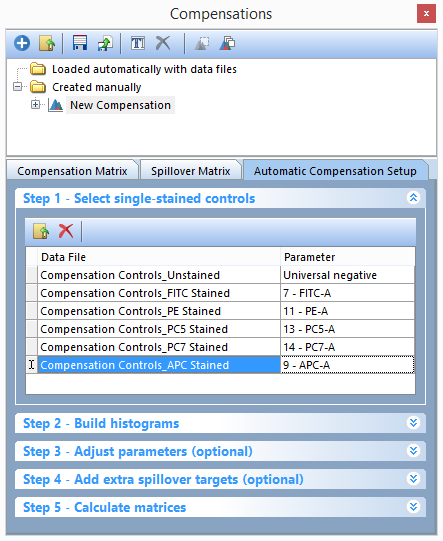
Figure T8.12 - All Parameters have been matched to their respective single stain control.fcs file.
13. Click on Step 2 - Build histograms to expand the build histograms window (T8.13).
14. Click on the Build Histograms button (T8.13).
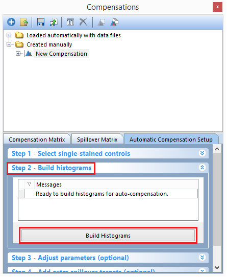
Figure T8.13 - The Build Histograms button will create a new page for scatter parameters and a new page containing a postive control and negative control histogram for each individual stain.
Six new pages will be created (Figure T8.14):
•Scatter Plot
•FITC-A control
•PE-A control, PC5-A control
•PC7-A control
•APC-A control
The Scatter Gate page contains a plot based on the first two parameters of the data while the rest of the pages (single stain control pages) contain two histograms for each parameter compensated. The top histogram shows the positive population from the single stain control for the parameter while the bottom histogram shows the negative population from the universal negative control. A histogram marker has automatically been created for each positive and negative population and each histogram marker has also been automatically converted and linked to a gate. All of the histogram markers/gates are children of the Scatter Gate which means adjusting the Scatter Gate will cause the histogram markers/gates to update in real time.
We will now make some adjustments to the Scatter Gate to refine the automatically marked/gated single stain and negative populations.
To better appreciate plot adjustments, turn on the Multiple Page view by:
15. Click on the View tab→Multiple Page→Two Pages (Vertical).
16. Select the Scatter Plot page for the left page.
17. Select the FITC-A control page for the right page.
your screen should now look as in Figure T18.14
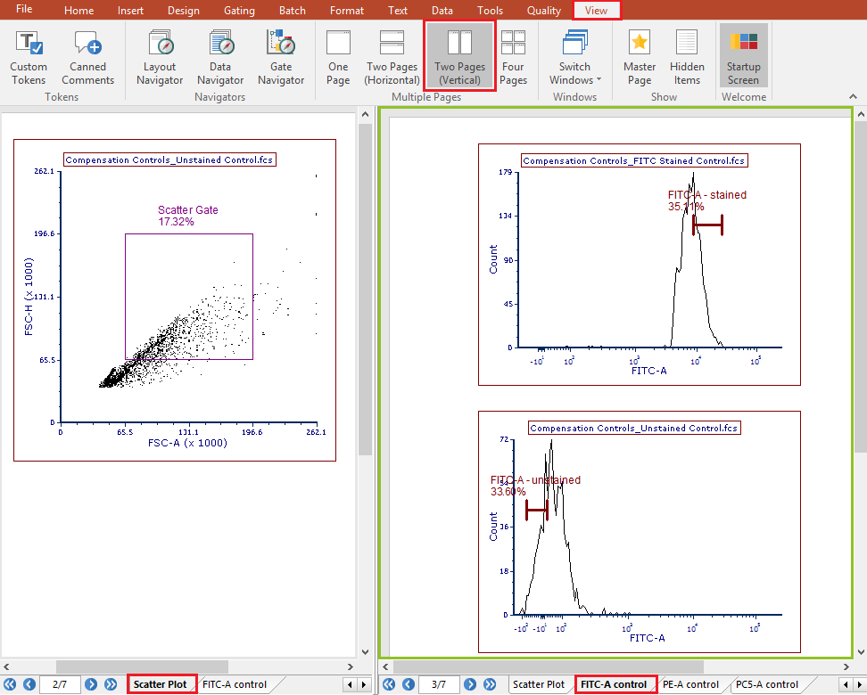
Figure T8.14 - Clicking on the build histograms button results in a Scatter Plot page and a new page with every single stained control.
In this instance FSC-H vs FSC-A are not the correct parameters for defining scatter so we will replace the Scatter Gate with a more appropriate one.
18. Change the X-Axis parameter on the Unstained Control dot plot (left page) to SSC-H (Figure T8.15)
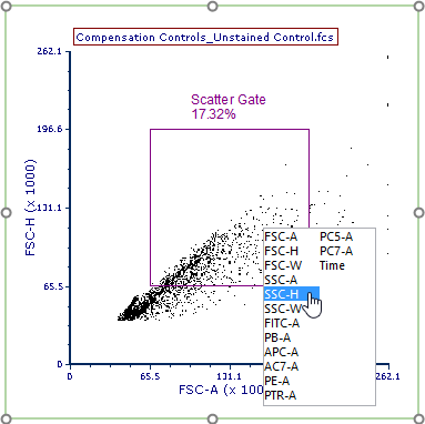
Figure T8.15 - Changing the X-Axsi parameter to SSC-H.
19. Choose the Gating tab→Create Gates→Rectangle.
20. Draw a gate around the beads population like the one in Figure T8.16 (left panel).
21. A Create New Gate dialog appears.
22. Chose the Replace an existing gate radio button (Figure T8.16).
23. Choose Scatter Gate from the bottom of the drop down list (Figure T8.16).
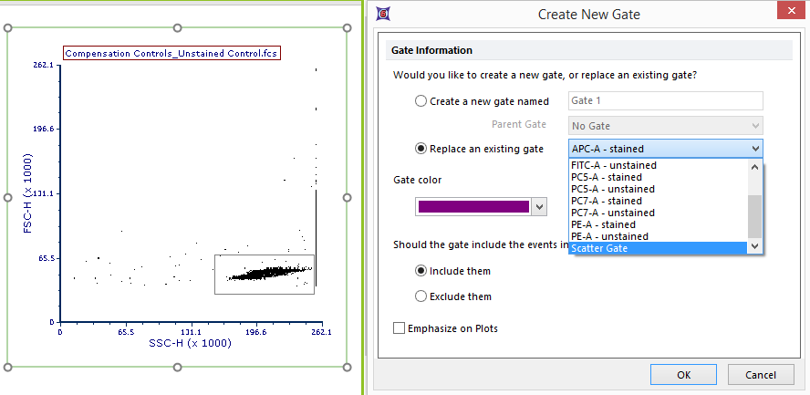
Figure T8.16 - Creating a gate around the bead population on the plot and choosing to replace the Scatter Gate with the newly created gate.
24. Click OK.
Notice that the original scatter gate has been replace with the new one you defined. It is convenient to replace the original scatter gate because all the single stained control histograms in the layout are already using that gate. If we had created a new gate, we would have had to apply that new gate to all the single stained control histograms. Notice that the subsequent single stain control histogram pages have updated to use this new gate.
User may also decide to refine markers position in the following pages of the layout (the ones containing single staining control histograms).
We will now complete the Automatic Compensation Setup in Step 5. Steps 3 and 4 of the Automatic Compensation Setup are optional and we will come back to them at the end of this tutorial.
25.Click on Step 5- Calculate matrices in the Compensations navigator.
26. Click on the Calculate matrices button (Figure T8.17).
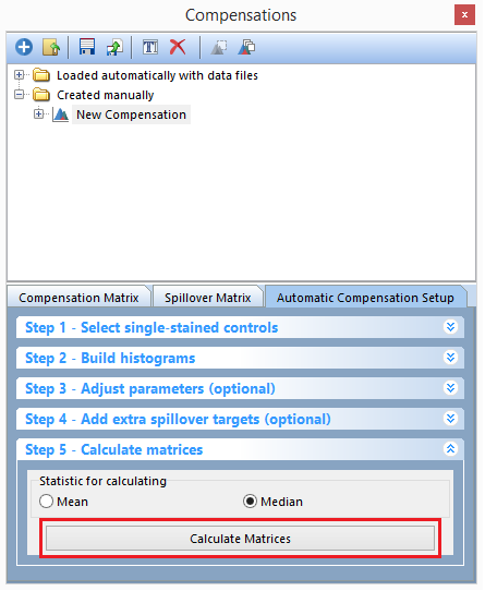
Figure T8.17 - Click the Calculate Matrices button to complete your automatic compensation setup.
All of the compensation and spillover matrix's will be automatically calculated and displayed in the Compensation Matrix and Spillover Matrix tabs of the Compensations navigator. The Editor view (highlighted in red) can be changed from Matrix Editor to List Editor to view the compensation definitions in matrix or list form (this may also be done in the Spillover Matrix tab). (Figure T8.18 below)
Note: Your values may differ slightly from figure T8.18 due to differences in how the scatter gate was manually setup in steps 20-25 of this tutorial.
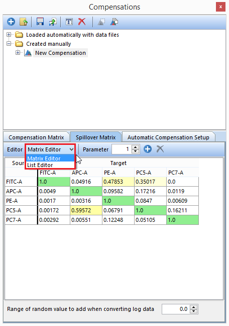
Figure T8.18 - The Spillover Matrix created from the Automatic Compensation Setup. The red box indicates you can change from Matrix Editor to List Editor view. The Spillover Matrix tab will display the spillover matrix for your compensation definition.
We will now switch back to a one page view and apply our new automatic compensation to a multicolor control.
27. Click on the View tab→Multiple Page→One Page.
28. Click on the Compensation Samples page tab to move on the first page of the layout (Figure T8.6).
29. Click on the New Compensation compensation in the Compensations navigator to select it (Figure T8.19).
30. Drag and drop (by click and holding the left mouse button) the New Compensation on top of the Compensation Controls_All Colors.fcs plot in the upper right of the layout (see red arrow in Figure 8.19).
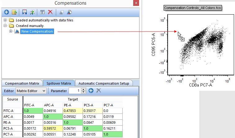
Figure T8.19 - Dragging the New Compensation definition from the Compensations navigator and dropping it on a plot will apply that compensation definition to the plot.
The plot will update and show the data properly compensated as in figure T8.20 below.
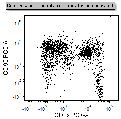
Figure T8.20 - The All Colors control plot with the compensation defined in the Automatic Compensation Setup feature applied.
Compensation and Spillover matrices may also be added anywhere in your layout or Microsoft Excel in a text box.
31. Click Compensation Matrix within the New Compensation definition to select it (FigureT8.21).
32. Drag the Compensation Matrix to an empty space in the layout and drop it (FigureT8.21).
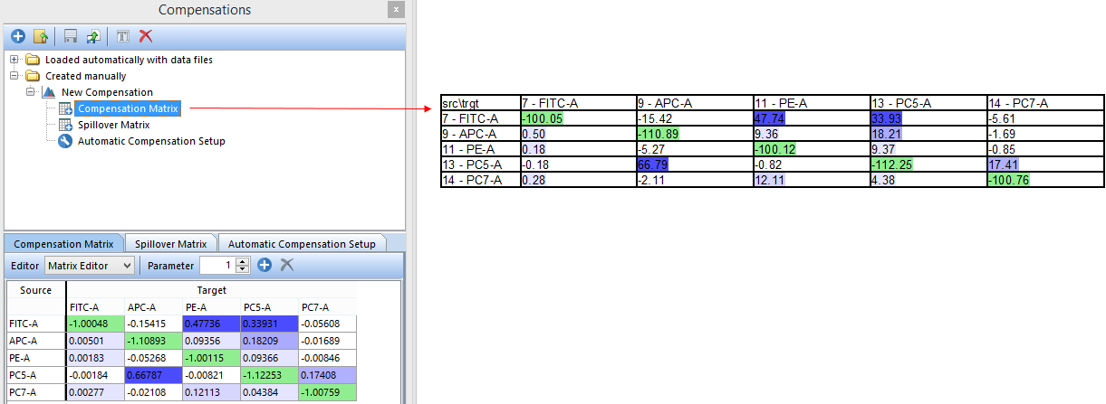
Figure T8.21 - Drag and drop the Compensation Matrix to a blank space in the layout (red arrow) to insert a text displaying all of the matrix values.
The compensation matrix will now be displayed in a text box (FigureT8.21). Steps 32 and 33 can be repeated with a drag and drop to Microsoft Excel if you would like the matrices displayed there.
At this point the Automatic Compensation Setup is complete although Step 3 - Adjust parameters (optional) and Step 4 - Add extra spillover targets (optional) may also be used to refine your single stain populations (Adjust parameters) or to have other targets defined without defining a source (Add extra spillover targets). If you would like to learn more about these advanced features please see the Automatic Compensation- Optional Steps 3 and 4 tutorial.
Please see the Manual Compensation tutorial or the Compensation section of the manual for more details on compensation in FCS Express.
Note: Sometimes when working with your own data digitization errors may occur as in Figure T8.22 below. This happens primarily if you are using log converted FCS 2.0 data. If you wish to correct for the digitization errors please see the brief Compensation Digitization Errors tutorial.
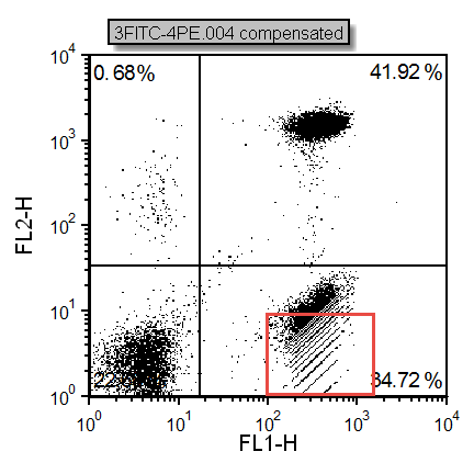
Figure T8.22 - Digitization errors after compensation can be seen in the red box. Please refer to the Compensation Digitization Errors tutorial to correct this type of error.
