In this tutorial:

•We will learn how to take Snapshots through the use of the Apply Iteration Snapshot tool.

•We will learn how to navigate through our data by using the Previous/Next buttons or through the Iteration drop down list on the Data tab.

•We will learn how to Flag an iteration for review later on during analysis.

•Although any data files of your own can be used to follow along in this tutorial, you have the option of using the same sample data files used in this tutorial. The sample data files are located in the Tutorial Sample Data archive.

 

1. Navigate to the Tutorial Sample Data folder from the File tab→Open.

2. Open the layout IterationSnapshots.fey.  

This layout contains 4 density plots and a 1D histogram and is currently displaying the first iteration of three loaded into the Data List.

3. Select the Batch & Export tab→Snapshots→Apply Iteration Snapshot button .

4. Click the Next button (double-headed right arrow) in the Data tab→Change Data on All Objects category to advance to the next iteration.

Alternatively, you can advance to the next iteration by selecting 2 from the Data tab→Change Data on All Objects→Iteration drop down menu, or by clicking 2 from the Iteration column in the Data List.

The content of the layout should now be similar to Figure T9.9.

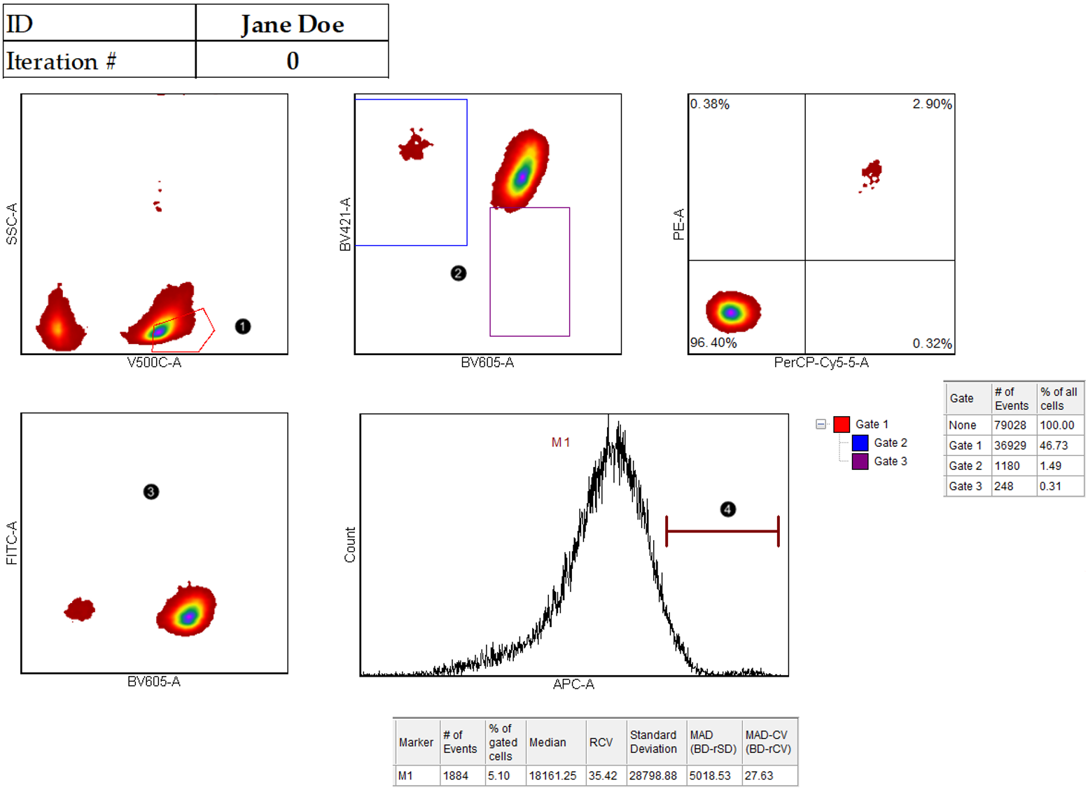
We now will make the adjustments for the 2nd iteration according to the steps below and as seen in Figure T9.9:

5. Adjust the red gate around the cluster on the SSC vs V500 plot (Figure T9.9, ).

6. Adjust the purple gate around the cluster in the right of the BV421 vs BV605 plot (Figure T9.9, ).

7. Right-click the FITC vs BV605 plot (Figure T9.9, ).

8. Choose Show Quadrants.

9. Adjust the M1 marker to capture entirely the peak on the APC 1D histogram (Figure T9.9, ).

 

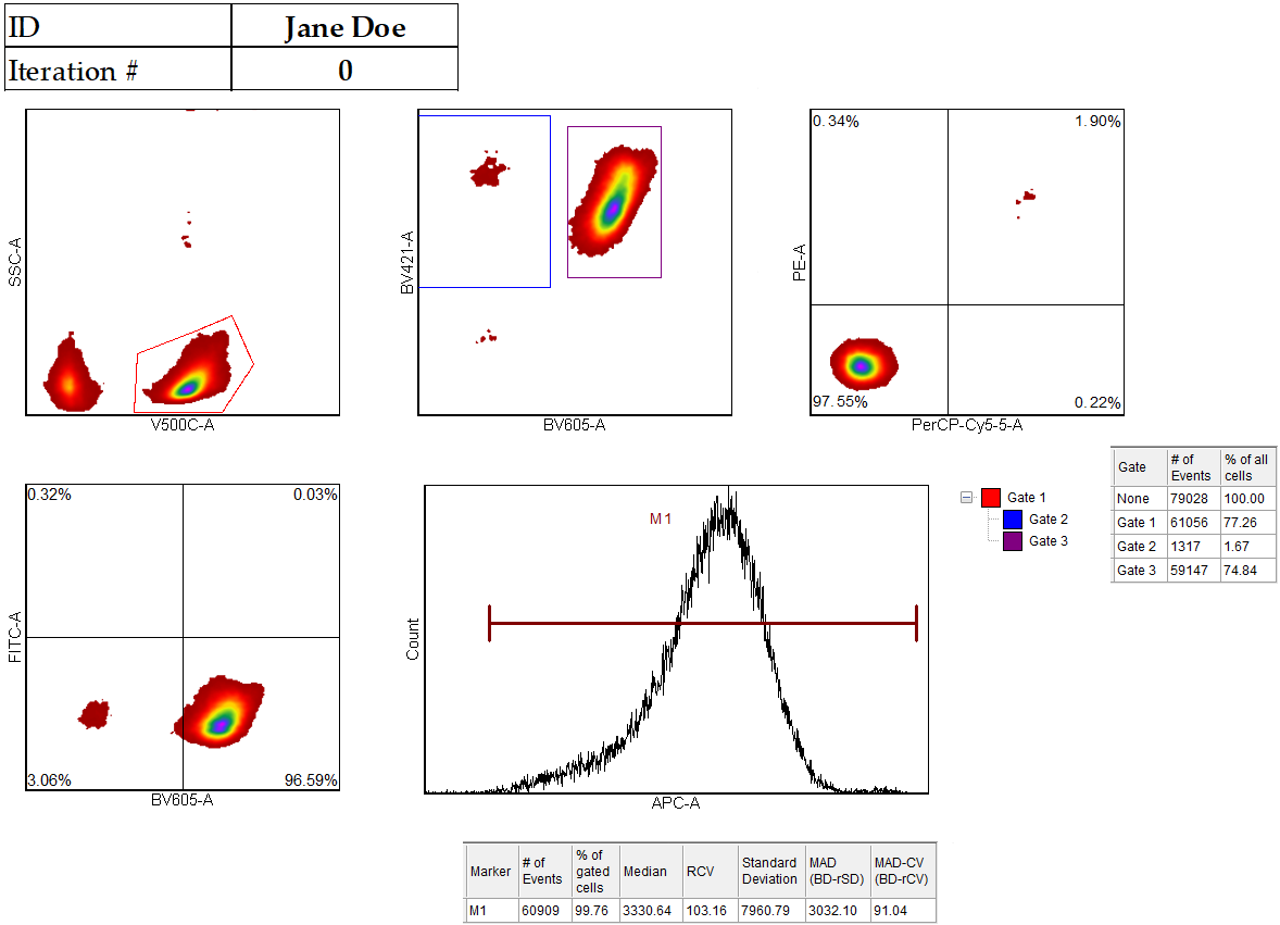
After these adjustments, the layout should resemble Figure T9.10.

We now will Flag the iteration for use later in the tutorial.

10. Click the Flag this Iteration button in the Data tab→Change Data On All Objects group (Figure T9.11, red outline).

 

 

Once the 2nd iteration is flagged, you will see a new icon within the Data List, next to the 2nd iteration: .

We will come back to the Flagged iteration in the next tutorial section, Batch Processing Snapshots.

11. Click the Next button (double-headed right arrow) in the Data tab→Change Data on All group to advance to the third iteration.

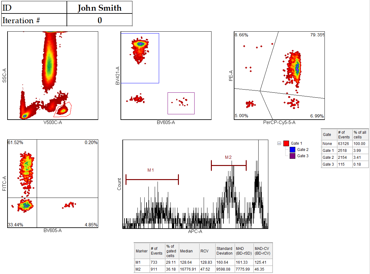
We now will make the adjustments for the third iteration according to the steps below and as seen in Figure T9.12:

12. Adjust the red gate around the cluster on the SSC vs V500 plot (Figure T9.12, )

13. Adjust the purple gate around the cluster in the lower right of the BV421 vs BV605 plot (Figure T9.12, )

14. Move the floating quadrant on the PE vs PerCPCy5.5 plot to a new position (Figure T9.12, )

15. Move the quadrant on the FITC vs BV605 plot to a new position (Figure T9.12, )

16. Move the M1 marker on the APC 1D histogram (Figure T9.12, ).

17. Create a new marker to accommodate the second peak on the APC 1D histogram (Figure T9.12, ).

 

The layout should now appear similar to Figure T9.13:

We will navigate back through our data to observe the Iteration Snapshot feature in effect.

18. Click the Previous button (double left hand arrow) in the Data tab→Change Data on All Objects group to move back to the second iteration.

19. Click the Previous button (double left hand arrow) in the Data tab→Change Data on All Objects group to move back to the first iteration.

Notice that FCS Express has automatically saved and applied a snapshot for each iteration.

20. Click on File tab→Save As to save your work.

21. Navigate to your desktop.

22. Name the layout file a name of your choice.

23. Choose Linked as the Data Link Style.

24. Click Save.

You can now double click on the layout file you saved in steps 20-24 to open and pick up your analysis where you left off.  After opening the saved layout you will notice clicking the Previous/Next buttons automatically applies the iteration snapshots saved with the layout.

In the next section, we will further investigate how Snapshots are integrated with Batch Processing.