Automatically Calculating Compensation Definitions
Instead of manually entering a value to subtract for every target-source pair, or guessing the compensation by eye using old-fashioned sliders, you can have FCS Express calculate the entire compensation definition for you. For step-by-step instructions on using the Automatic Compensation Setup please see our Automatic Compensation Tutorial. To get started, use the Data tab→Data Info→Compensations command, open the Compensations navigator, and add a new compensation with the Create a new compensation button ![]() . You can then click on the Automatic Compensation Setup tab to access the automatic settings (Figure 16.9).
. You can then click on the Automatic Compensation Setup tab to access the automatic settings (Figure 16.9).
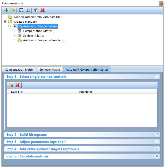
Figure 16.9 The Automatic Compensation Setup tab.
The Automatic Compensation Setup tab contains 5 steps to calculate your compensation. Step 3 and step 4 are optional and do not have to be completed.
| • | Step 1 - Select single-stained controls (Figure 16.10) |
In order to automatically calculate the compensation definition, you will need an .fcs file with a single stain control for each parameter you wish to compensate and an unstained control. The unstained control can be a universal negative, a negative population defined by a gate, or the negative population with the tube of the positive control. You will also have the option of using an unstained control for each parameter you wish to compensate or to use populations defined in user-created gates in Step 3: Adjust parameters.
| 1. | Click the Add data for auto compensation button, |
| 2. | Choose the parameter that was stained for each control sample and the universal negative using the Parameter dropdown menu. |

Figure 16.10 Step 1 - Select single-stained controls. Add compensation control data files and choose their respective channels from the Parameter drop down list.
| • | Step 2: Build Histograms (Figure 16.11) |
| 1. | Click the Build Histograms button. If there was something wrong with the files or parameters you selected in the previous step, an error message will appear here to let you know what the problem was, and the Build Histogram button will be disabled until the error is corrected. |
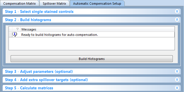
Figure 16.11 Step 2: Build Histograms
If there were no errors, the Ready to build histograms for auto-compensation settings message appears in the Build histograms dialog. The Build histograms step will automatically create the following items (Figure 16.12):
| • | Scatter Plot Layout Page: A page will be created with a plot displaying SSC vs FSC and a Scatter Gate. The Scatter Gate is automatically created and used to define the "live" cells or cells of interest in your compensation controls. All of the fluorescence gates are children of the Scatter Gate, which means adjusting the Scatter Gate will cause all other gates to update in real time. If the Scatter Gate does not appear on the right parameters (e.g., SSC-H vs FSC-H), change the gate using the replace gate feature. To replace the Scatter Gate with a new gate: |
| . | Change the X and Y axes to the correct parameters. |
| . | Draw a gate around the population of interest. |
| . | Choose the Replace an existing gate radio button in the Create New Gate dialog. |
| . | Select Scatter Gate from the drop down menu. |
| . | Click OK. |
(Note: These steps are also described in the Automatic Compensation Setup tutorial.)
| • | Single Stained Control Layout Pages: A new page will be created for every parameter you are compensating (e.g., "FITC-A control", "PE-A control" in the image below). The page will display one histogram with the stained population marked and one histogram with the unstained population marked. Markers will be placed based on FCS Express auto recognition of peaks, but can be adjusted. |
Note: the unstained population histogram will only appear if a universal negative is chosen. If it was not, only a single plot with two markers (for positive and negative populations) will appear.
| • | Gates: New gates will be created for the Scatter Gate and each stained and unstained set up markers will be converted and linked to gates. After the initial "auto-gating" all the gates and markers created in the Build histograms can be manually adjusted. (Note: A Gate View will not automatically be inserted.) |
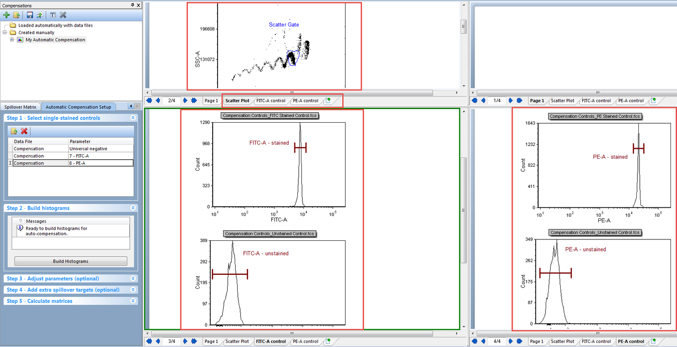
Figure 16.12 Layout after Step 2 of Autocompensation setup. Note the Scatter Plot, FITC control, and PE control pages. Also notice that a plot for SSC vs FSC has been created with a Scatter Gate automatically applied. Histograms with markers for the stained and unstained populations have also been automatically created.
This step is rarely used, but can be helpful with certain kinds of data (e.g., where the Stained or Unstained population must be defined on a different plot). Once you have determined your initial compensation parameters via Step 1 and Step 2 (or completed your compensation matrix in step 5) you can add Adjust parameters in Step 3.
Step 3 - Adjust parameters (optional) is useful when you would like to refine the populations that are used for calculating compensation. Dragging and dropping new plots, files, or gates in this section will allow you to override the automatic setup and use gates and plots of your choice. For instance, if the Automatic Compensation Setup does not make a good estimate of the population or if you would like to use a population from another file, gate, or plot, Step 3 would be useful. Parameters may be adjusted or changed altogether by dragging and dropping a plot or gate onto the parameter for the Stained and Unstained columns. If a gate is dropped, the compensation definition will be based on that gate, including its hierarchical position visible in the Gate View object. If a plot is dropped, the compensation definition will be based on the entire population on the plot. If you have adjusted a parameter after the matrix has been calculated you must click on the Calculate matrices button in Step 5 again to apply the change.
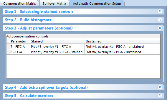
Figure 16.13 The Adjust parameters dialog displaying the currently defined parameters, plots, and gates.
Instructions for adjusting parameters (Figure 16.14):
| 1. | Click and hold on a gate or plot. |
| 2. | Drag the gate or plot to appropriate cell in the Autocompensation controls table (red arrow). |
| 3. | Release the mouse button. |
The new gate and or plot will appear by name in the appropriate cell in the Autocompensation controls table of the Adjust parameters pane (Figure 16 below, green arrow).
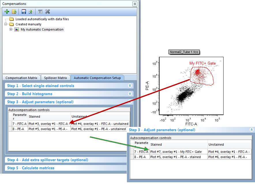
Figure 16.14 To change a parameter plot or gate drag the gate or plot onto the plot you wish to change. The plot information will then update to the newly choosen gate or plot.
Adding extra spillover targets allows you to have other targets defined without defining a source. This is useful if you would like to have an idea of what spillover would look like if an extra parameter was added in future experiments. To add an extra spillover target simply check the box for the extra target you would like to add. Note: extra spillover targets will only appear for parameters that were acquired with the data.
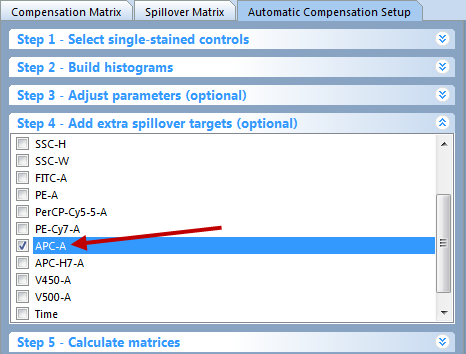
Figure 16.15 The Add extra spillover targets (optional) dialog. Checking a box will calculate the spillover for targets that have no source.
| • | Step 5: Calculate matrices (Figure 16.16) |
In this final step you can choose to Calculate Matrices based on the Mean or Median depending on your preference for your data and experiment. Click on the radio button for either choice to apply your preference.
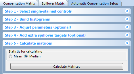
Figure 16.16 Step 5: Calculate Matrices button and choosing Mean or Median.
Your Compensation Matrix will then appear in the Compensations navigator (Figure 16.17)and you may edit any of the source-target pairs through the Compensation Matrix, Spillover Matrix, or make new adjustments in the Automatic Compensation Setup.
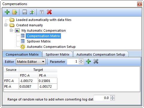
Figure 16.17 The Compensation Matrix after the Automatic Compensation Setup is complete.
The automatic compensation setup settings are saved with the layout. To create another compensation matrix from a different set of data, simply add a new compensation with the Create a new compensation button ![]() and begin the Autocompensation setup process again.
and begin the Autocompensation setup process again.
We also suggest that you use the compensation determined in the Automatic Compensation Setup and apply it to different layouts and files rather than re-creating the same compensation definition many times.
A step-by-step description of the Automatic Compensation Setup feature is provided in our tutorials at Compensation Tutorial.
