Create a Custom Data Table
We will now use the Custom Tokens of the titration ratios to create a custom data table of the CD64 concentration (volume) versus the CD64 staining of the Monocyte/Lymphocyte population. A custom data table is similar to a spreadsheet, where you can create and edit cells. At anytime if you would like to skip ahead to the Insert a Scatter with Regression Plot section the steps from the tutorial have been completed in a new layout for the next section.
We will begin by inserting a new blank page on the layout you created in the previous section. You may also begin this tutorial by opening the layout Titration_Custom_Tokens_Complete.fey found in the FCS Express Sample Data folder which has all the steps from the Define Custom Tokens tutorial completed.
| 1. | Select the Insert→General→New Page command (Figure T17.20). |
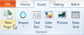
Figure T17.20 Insert New Page
A blank new page will appear. We will now change the view so that we can view both pages at the same time.
| 2. | Select the View→Multiple Pages→Two Pages (Vertical) command (Figure T17.21). |

Figure T17.21 View Two Pages
Both layout pages now appear as shown in Figure T17.22 with Page 2 to the left of Page 1.
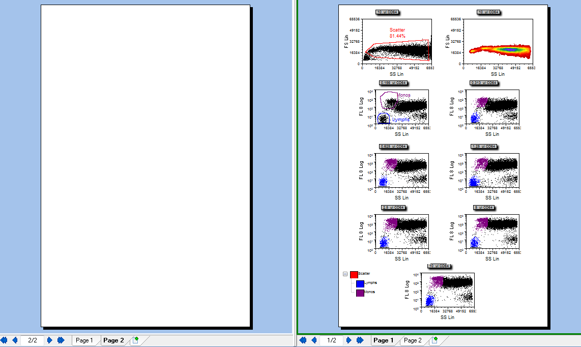
Figure T17.22 Both Layout Pages
We will now insert a custom data table onto Page 2 of the layout.
| 3. | Select the Data tab→Save/Load→Custom Data→New Custom Data command (Figure T17.23). |

Figure T17.23 Selecting the New Custom Data Command
The Create new custom data dialog appears, similar to Figure T17.24.
| 4. | Type 'Titration CD64' in the title window. |
| 5. | Change the Columns value to '2'. |
| 6. | Change the Rows value to '7'. |
| 7. | Click OK. |
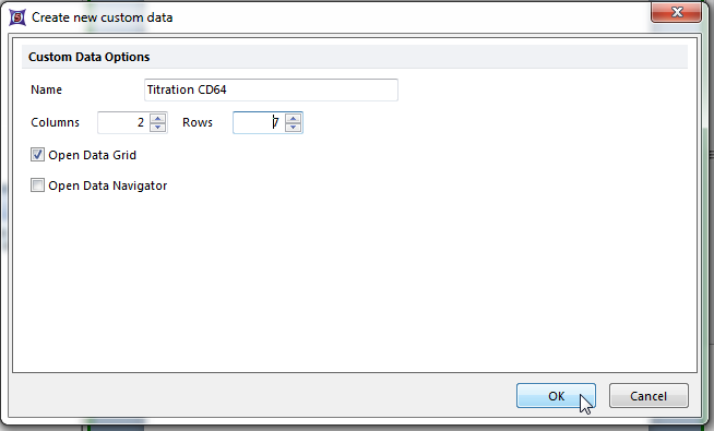
Figure T17.24 Create New Custom Data Dialog
A custom data table appears on Page 2 of the layout. We will now format the table to put in appropriate column names.
| 8. | Click on the column labeled 'A', shown highlighted in blue in Figure T17.25. |
| 9. | Right-click to bring up the pop-up menu. |
| 10. | Select Rename Selected Column from the pop-up menu. |
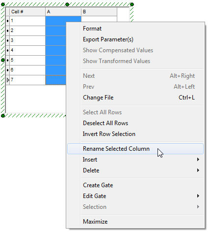
Figure T17.25 Rename Selected Column Menu Item
The New Column Name dialog appears, similar to Figure T17.26.
| 11. | Type 'volume [ul]' in the Enter the new name for column A window. |
| 12. | Click OK. |

Figure T17.26 New Column Name Dialog
The custom data table updates to reflect the new column name. We will now repeat steps 9 – 11 for column B.
| 13. | Click on the column labeled 'B'. |
| 14. | Right-click to bring up the pop-up menu. |
| 15. | Select Rename Selected Column. |
| 16. | Type 'M/L ratio' in the Enter the new name for column B window of the New Column Name dialog. This is the Monos/Lymphs ratio we defined in the custom tokens. |
| 17. | Click OK. |
The columns of the custom data table are now appropriately labeled as shown in Figure T17.27.
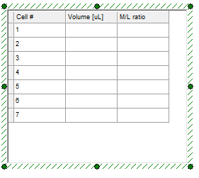
Figure T17.27 Custom Data Table with Column Names
We will now fill the custom data table with the appropriate values, by dragging and dropping the appropriate plot onto the custom data table. The volume column of the custom data table will be filled using the keyword conc, found in the data file, which refers to the volume of CD64 used. We could directly type the volume into the custom data table. However, using the keyword token conc provides more flexibility for analysis, yielding a generic template that can be used for future titration experiments. If you have another titration experiment with seven concentrations, which uses the monocyte:lymphocyte staining ratio and a conc keyword, you will be able to load the data files into this layout and directly use the custom token and custom table definitions.
| 18. | Place the cursor over the plot of 0.156 ul CD64, shown with red border in Figure T17.28. |
| 19. | Press and hold the left mouse button and drag the plot onto the custom data table. |
| 20. | Release the mouse when the cursor is on the top cell of the volume [ul] column, indicated by the cursor in Figure T17.28. |
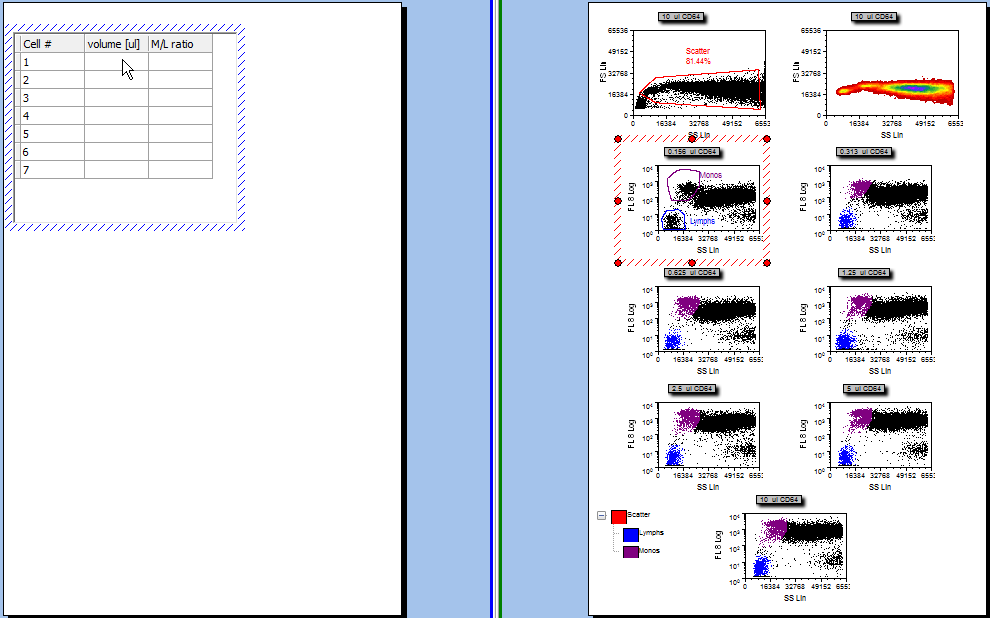
Figure T17.28 Dragging and Dropping the 0.156 ul CD64 Plot onto the Custom Data Table
The Paste Special dialog appears, shown in Figure T17.29. All the data files have a keyword 'conc' that specifies the volume of CD64 used for staining.
| 21. | Select keyword token, shown highlighted in Figure T17.29. |
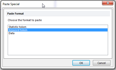
Figure T17.29 Keyword Token in the Paste Special Dialog
The Edit Keyword dialog appears, similar to Figure T17.30.
| 22. | Type 'conc' in the Select a keyword: field, indicated by the cursor in Figure T17.30. |
| 23. | Click OK. |
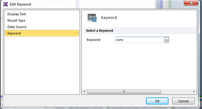
Figure T17.30 Edit Keyword Dialog
The first cell of the volume column, in the custom data table, updates to reflect the entry of the keyword conc, which contains the value of 0.156. We will now copy the keyword token entry and paste it into the next cell in the volume column.
| 24. | Click on 0.156, shown highlighted in blue in Figure T17.31. |
| 25. | Select the text 'Keyword: conc for Plot #3, overlay #1', shown highlighted in gray in the cell editor (Figure T17.31). Note: whenever you click on a cell, the cell editor appears allowing you to edit the current contents of the cells. |
| 26. | Copy the text using Ctrl+C on the keyboard. |
| 27. | Click inside the next cell in the column, indicated by the cursor in Figure T17.31. |
| 28. | Place the cursor in the editor window (it should be empty). |
| 29. | Paste the text using Ctrl+V on the keyboard. |
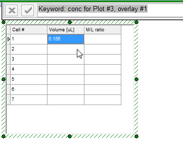
Figure T17.31 Copying and Pasting the Conc Keyword
We will now edit the keyword token to use the 0.313 μl CD64 plot.
| 30. | Double-click on the text 'Keyword: conc for Plot #3, overlay #1'. |
The Edit Statistic page Data Source category appears, similar to the Create Statistic dialog previously shown in Figure T17.9.
| 31. | Select Color Dot - 0.313 ul CD64.fcs.DNS (SS Lin vs. FL 8 Log). |
| 32. | Select OK. |
Repeat steps 27 through 32 for the other entries of the volume column using the other five remaining data plots, 0.625 μl CD64 through 10 μl CD64. The custom data table should look similar to Figure T17.32.
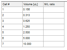
Figure T17.32 Custom Data Table with Volumn Values
We will now enter the values for the M/L ratio column, which represent the Monos/Lymphs ratio, by dragging and dropping the custom ratio tokens we previously defined onto the M/L ratio column of the custom data table.
| 33. | Place the cursor on the 0.156 ratio in the Custom Tokens window, highlighted in blue in Figure T17.33. |
| 34. | Press and hold the left mouse button while dragging the 0.156 ratio over to the custom data table. |
| 35. | Release the button when the cursor is over the top cell of the M/L ratio column, indicated by the cursor in Figure T17.33. |
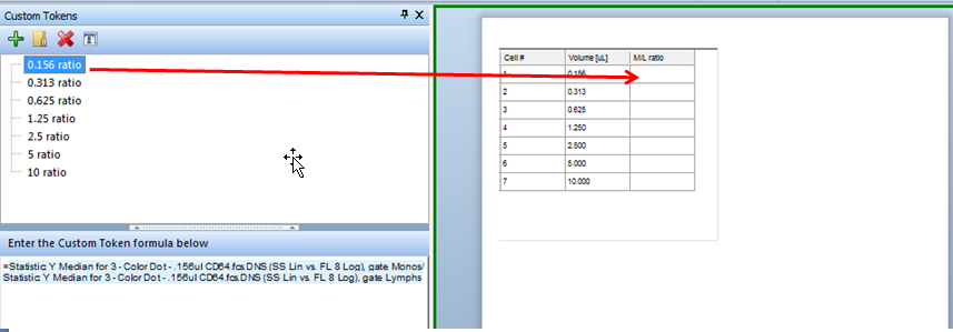
Figure T17.33 Dragging and Dropping the Custom Token onto the Custom Data Table
When the mouse is released, a Paste Special dialog box will appear, as shown in Figure T17.34.
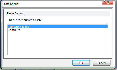
Figure T17.34 Paste Special box - Text with Tokens
The custom data table is now updated to show the ratio of Monocytes to Lymphocytes for the 0.156μl concentration of CD64, as shown in Figure T17.35.
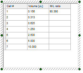
Figure T17.35 Custom Data Table Updated with 0.156μl Data
Repeat steps 33 through 35 for each of the custom token ratios, 0.313 through 10, to fill in the M/L ratio column on the custom data table. The custom data table should now look similar to Figure T17.36.
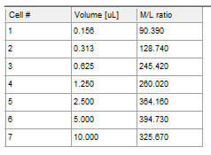
Figure T17.36 Final Custom Data Table
In examining the custom data table, one can see that the largest Monos/Lymphs ratio is obtained using 5μl of CD64. In the next section, we will insert a scatter with regression plot of this data so that we can better display the titration curve.
