Getting Started with Image Cytometry

Contents
In this section, we will learn how to:
| • | Understand the required components for importing image data |
| • | Load a layout with image data |
| • | Modify and insert new data plots and images using picture plots |
| • | Apply example image gating approaches |
| • | Create a data grid to and include cell images to create a "cell gallery" |
| • | Visually examine and optimize control settings for a Nuclear Translocation assay |
| • | Modify settings and gating for the data grid displaying a cell gallery |
Understanding Image Data Import with FCS Express 5 Image Cytometry
When working with image data we have several components of data to consider, the raw image data, the segmentation maps used to specify individual objects within the image, and derived per-object multi-parametric results. Ideally, the data you will work with has all of these components available to FCS Express 5. With only the cell by cell multi-parametric data you can still review results with all of the familiar flow analysis tools without interactive image options.
If the images and segmentation maps are available, FCS Express can link your multi-parametric results back to the source images. The individual cells can then be highlighted in Picture Plots, images of single cells can be excised and displayed in cell galleries, and meaningful multi-parametric data can be reviewed on a cell by cell basis. FCS Express 5 Image Cytometry is able to import data from a number of imaging platforms so you can easily import and work with your data.
Section 1: Working with Image Cytometry Data
We will be using the IntroToImage1.fey layout for this section which is located in the Tutorial Sample Data archive→Intro to Imaging Tutorial folder. This layout contains a detailed pre-formatted approach to working with image data. As an introduction to use of the image cytometry features we will not go into detail for operations that are detailed in our other general tutorials. Relevant detailed tutorials will be referenced as applicable.
| 1. | Load the IntroToImage1.fey layout from within the "Intro to Imaging Tutorial" folder within the Tutorial Sample Data archive. The multi-parametric data and images are embedded in this layout. |
This is a 2-page layout, please confirm you are viewing page Example page. This page contains three Picture Plots and a Color Dot Plot of the cellular data (Figure T28.1). It also has the "Data List" indicating data used in the layout, and a "Data Grid" displaying single cell information to the right side of the work area on the page. You can place plots and grids anywhere in the layout on the Example page. The layout also contains a Blank page.

Figure T28.1 Overview of the IntroToImage1.fey layout
The Dot Plot displays two of the many parameters measured and saved by CellProfiler plotted against each other on the X-Y Axes. You can change the parameters displayed on the Dot Plot easily. We will proceed by changing the X-Axis parameter.
| 2. | Press and hold the left mouse button down over the X-Axis label of the Dot Plot. You will see a menu of parameters appear (Figure T28.2). |
| 3. | Scroll through the list of parameters left or right by moving the mouse to the left or right of the list box, while holding down the mouse button. |
| 4. | Move the mouse until the parameter you wish to change to is highlighted. |
5. Release the mouse button.
The new parameter will now be selected and displayed on the X-axis. This will work on all plot types with multi-parametric data.

Figure T28.2 Selecting a New Parameter on a 2d Plot.
Undo is a powerful feature in FCS Express 5. Note that once you have made and change you can use CTRL+Z to undo your changes any time you like. FCS Express 5 supports unlimited undo commands.
| 6. | Type CTRL+Z to undo the new parameter for the X-Axis. |
There is an alternative way to change X-Y Axes parameter display and have access to change other qualities of the Dot Plot:
| 7. | Right click on the Dot Plot. |
| 8. | Select Format from the pop-up menu (Figure T28.3). |
This is the general format screen for the plot. All plots and many other objects in FCS Express may be formatted similarly.

Figure T28.3 Launching the Format Menu for a Plot
Observe that you now have a number of options for changing the plot. Formatting all characteristics of the plot are possible.
The X and Y Parameters can be changed in this manner as well. We will access many features in the Formatting menu during this tutorial, so please familiarize yourself with the various items in the menu, but do not make any changes at this time.
| 9. | Choose the Overlays category (Figure T28.4). X and Y Parameters can be easily changed here (red rectangle in Figure T28.4). |
For the moment let's take advantage of this windows to change Dot Size to 8 (Figure T28.4).

Figure T28.4 The Format Sub Menus
| 10. | Increase the Dot size to 8. |
| 11. | Click OK to accept the change. |
| 12. | Select the Gating tab→Create Gates→Rectangle. (Figure T28.5) |

Figure T28.5 Selection of Gate Type
| 12. | Press and hold the left mouse button down on the center of the Dot Plot. |
| 13. | While holding the left mouse button down, drag to the right and down to draw a rectangular gate on the dot plot (Figure T28.6). |
| 14. | Release the mouse button when the gate is the desired size. |

Figure T28.6 Drawing a Rectangular Gate
| 15. | Enter the name "Cells Gate 1" when the Create New Gate dialog appears (Figure T28.7). |

Figure T28.7 Create New Gate
| 16. | Click OK. Notice that the cells included in the gate change to appear in red in both picture plots (Figure T28.8). |

Figure T28.8 Highlighting of Cells Included in Cells Gate 1
Recall that Unlimited Undo and Redo is a powerful feature in FCS Express 5. Note that once you have made changes you can use CTRL+Z to undo your changes if you like.
| 17. | Type CTRL+Z to undo the addition of Cells Gate 1. |
| 18. | Type CTRL+Y to redo the addition of Cells Gate 1. |
| 19. | Click once inside the Cells Gate 1 on the dot plot. This selects the gate. In a selected rectangle gate, the corners will appear with blocks on them. These blocks are "vertices" and they are the point you can grab to change the gate dimensions. |
| 20. | Press and hold the left mouse button over one of the vertices of Cells gate 1. |
| 21. | Move the mouse leftward and downward (in the direction of the red arrow in Figure T28.9) until the gate is similar in size to that shown in Figure T28.9 below. |

Figure T28.9 Increasing the Size of Cells Gate 1
| 22. | Release the mouse button. Notice the increased gate size include more cells in the gate which also means more cells become highlighted in red in the images (Figure T28.9). You can also move a gate. |
| 23. | Press and hold the left mouse button inside the gate (but not over one of the vertices) Figure T28.10. |
| 24. | Move the mouse with the left button depressed to place the gate in a new location. |
| 25. | Release the mouse button when the gate is in the desired position. |
Observe the highlighted cells in the picture plots changing to, or from, a red color as you modify or move gates to indicate which cells are in the gate.

Figure T28.10 Moving Cells Gate 1
| 26. | Close the layout and do not save changes. |
Section 2: Building a Layout Page From Scratch
| 27. | Open IntroToImage1.fey. We will build up the Example page from scratch. |
| 28. | Click on the Blank Page Tab. (Figure T28.11) |
Figure T28.11 Selecting the Blank Page Tab
| 29. | Click Insert tab→Insert 2D plots→Picture Plot |
| 30. | Press and hold down the left mouse button to drag and drop a square anywhere on the blank page. This will insert a Picture Plot with images of the cells (Figure T28.12). |

Figure T28.12 The Inserted Picture Plot
The picture plot will be called pictureplotsample1.dns. This is because this data is embedded in the layout as indicated by the Data List shown in the layout (Figure T28.13). (Note that "pictureplot1.dns" may not be highlighted in dark blue on your layout, and that is fine)

Figure T28.13 The Data List
| 31. | Select the pictureplotsample1.dns Picture Plot by clicking on it. |
| 32. | Copy (CTRL+C) the pictureplotsample1.dns Picture Plot |
| 33. | Paste (CTRL+V) pictureplotsample1.dns just below the original on the same page. |
You will have two identical plots one above the other as shown in Figure T28.14.

Figure T28.14 Copy and Paste a Picture Plot
| 34. | Change the X-Axis label on the pasted Picture Plot from Cytoplasm to DNA (Figure T28.15) as described previously in step 2 or steps 7-9. |
You should now have the Cytoplasm (green) and Nuclear (Blue) image as in Figure T28.15 below.

Figure T28.15 Changing the Image Parameter of a Picture Plot
| 35. | Click anywhere that is empty on the layout. Paste pictureplotsample1.dns plot again in the upper right part of the page. |
| 36. | Click on the Picture Plot in the lower left that is displaying the DNA image plot to place it in edit mode. (Ensure the green selection box surrounds the plot, as shown in Figure T28.15 above). |
| 37. | Click on the green border of the Picture Plot to place it in Selected mode (the border became red colored). When plots are in selected mode, you can move then or resize them etc. |
| 38. | Press and hold the left mouse button while the mouse is over the red border of the Picture Plot displaying the DNA image. |
| 39. | Move the mouse until the outline of the DNA plot is over the top right cytoplasmic plot. You will know you are in the right spot when the "+" appears next to the cursor and the borders of the plot turn blue (Figure T28.16). |

Figure T28.16 Drag and Drop a Picture Plot onto Another Picture Plot to Create a 2d Overlay
A Paste Special dialog will appear as see in Figure T28.17 below.
| 40. | Select "2D Plot Overlay(s)". |
")
Figure T28.17 Selecting 2D Plot Overlay(s)
| 41. | Click OK. |
This will create a two channel overlay as shown in Figure T28.18.

Figure T28.18 Completed 2D Overlay
Notes:
To learn other ways to load a new image data set and insert image plots see the Picture Plots tutorial.
To learn more ways to modify the data and image plots see the Formatting Plots tutorial.
We will now insert a 2D Dot Plot in the layout
| 42. | Click on Insert Tab→Insert 2D Plots→Dot (Figure T28.19). |

Figure T28.19 Selecting the Dot Plot Icon
| 43. | Right click on the Dot Plot to open the Format Window in order to change from the default display (Figure T28.20). |

Figure T28.20 Default Configuration of Inserted Dot Plot
| 44. | Select Format. |
| 45. | Choose the Overlays category. |
| 46. | Set the X Parameter to Intensity_IntegratedInstensity_Cytoplasm as shown in Figure T28.21 below. |
| 47. | Set the Y Parameter to AreaShape_Area also shown below in Figure T28.21. |
| 48. | Increase the Dot size from 1.0 to 10 (Figure T28.21). |
| 49. | Click OK. |
Figure T28.21 Format Settings for New Dot Plot
The Dot plot will now appear as in Figure T28.22.

Figure T28.22 Formatted Dot Plot
| 50. | Insert a gate by selecting Gating tab→Create Gates→Rectangle as you have done previously in the tutorial (Steps 11-14). |
| 51. | Name the gate Cells Gate 1. |
| 52. | Click OK. |
Your Blank page will now look the same as the Example Page as in Figure T28.23.

Figure T28.23 Completed Example Page
| 53. | Close the layout, and do not save changes. |
Section 3: Image Gating Strategies
When using image cytometry data it can be very useful to apply gates to dot pots representing cellular data and review the gated cells in the original images. Reviewing the actual images of cell helps confirm that the gated populations represent the expected changes in cell morphology. In this section we will 1) gate on cells in an image and update plots and 2) gate on plots to update highlighted cells in images.
| 54. | Load the IntroToImage2.fey layout from the Tutorial Sample Data archive→Intro to Imaging Tutorial folder. |
This layout has a two Picture Plots and two color Dot Plots of the cellular data from a nuclear translocation assay. The images represent the nuclear stain and cytoplasmic stains of the same cells (Figure T28.24). Notice the gates on the cytoplasm image. The gates appear as a green square and red circle. Notice the red and green dots in the color dot plot below the image which indicates the cells that are within the gates on the Picture Plot. Note that we have also included a Gate View and Cell Gallery in the layout. These help us keep track of activity in the layout. Items not yet discussed are labeled in red. Figure T28.26 below displays the complete layout.

Figure T28.24 Complete Layout view for IntroToImage2.fey
| 55. | Select and move the green square and red circle gates shown in Figure T28.25. Observe the red and green dots updating in real time on the Dot Plot below the image to indicate which cells are in the gates. |
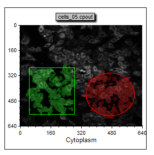

Figure T28.25 Dot Plot Displaying Gated Cells in Color
Notice the Cyan Square gate on the Nuclear Image dot plot on the lower right side of the page (Figure T28.26). Notice how the cells in the nuclei_05.cpout Picture Plot are highlighted in cyan when they fall within the cyan square gate.
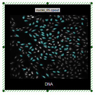

Figure T28.26 Cell Within Cyan Square Gate are Higlighted
| 56. | Select, move, and increase the size of the Cyan Square Gate on the plot. |
Notice the cyan cells updating in the DNA image in real time.
| 57. | Drag and drop the Green Square gate from the Cytoplasm Picture Plot onto the DNA Picture Plot with cyan cells as shown in Figure T28.27. |

Figure T28.27 Drag and Drop a Gate to Another Plot
Notice that the only cells that appear cyan are those that fall in the Green Square gate. The DNA picture plot is only highlighting cells within the cyan gate and since the Green Square gate has been applied the plot now only displays highlighted cells that fall within the combined cyan gate and the green square gate (Figure T28.28a and b).

Figure T28.28a Venn Diagram of Combined Green Square and Cyan Gates

Figure T28.28b Highlighted Cells Are Within Combined Gates
| 58. | Press CTRL+Z to undo applying the Green Square gate to the nuclei_05.cpout picture plot. |
| 59. | Drag and drop the Cyan Square gate from the Nuclear Image dot plot onto the DNA picture plot to reset the gate applied to be Cyan Square. |
Notice that only the gated cells remain visible in the image (Figure T28.29). (The display may not change since the cyan gate was applied prior to adding the green gate)

Figure T28.29 Cells within Cyan Gate Highlighted on Picture Plot
Notice the Data Grid displaying cell images. The images of cells provide a "Cell Gallery" on the right side of the layout displaying all cells in the image with the selected parametric data. Notice that the gate within which a cell resides is displayed by a colored rectangle in the Gates column (See Figure T28.30 below).
| 60. | Drag and drop the Cyan Square gate from the Nuclear Image dot plot onto the Data Grid. |
Notice the cell gallery component of the Data Grid now only displays the cells in the Cyan Square gate. Cells in the Cyan Square gate that are also in the Green Square and/or Red Circle are also indicated (you may have to scroll down to see them). Note that depending on the last position of the gates in the demo layout your Data Grid may not appear exactly as in Figure T28.30.

Figure T28.30 Example of Data Grid with Cyan Gate Applied
| 61. | Move the Cyan Square gate to a new location on the DNA picture plot and watch the cells in the gallery and picture plot update. |
| 62. | Left Click on the Data Grid displaying the cell gallery to select it. |
| 63. | Right click on the Data Grid and select Format to open the format window for the cell gallery. |
| 64. | Click Parameters to Display. |
| 65. | Scroll down the list and Click the check boxes next to Location_Center_X and Location_Center_Y to select them to be displayed in the cell gallery (Figure T28.31). |

Figure T28.31 Selecting Parameters to Display in Data Grid
| 66. | Click OK. |
Notice that the cell gallery is now displaying the selected variables. The expand the size of the data grid to see everything. You may expand column headers can be expanded in the live software view if names are long. The cell images are displayed as a result of selecting the check boxes for the image names Cytoplasm and DNA at the bottom of the list (Figure T28.32). We will refer to adding cell images to a data grid as adding a "Cell Gallery" to a data grid.

Figure T28.32 Formatted Data Grid With Added Parameters
| 67. | Close the layout do not save changes. |
Notes: To learn more about Gating options see the tutorial called "Gating".
Continue to the next topic - Using the High Content Module with Image Data.