R Cluster Transformation
Customized cluster analysis can be applied to a file of interest using the R Cluster Transformation input method.
To be compatible with the method, the Execute function defined in the R script should result in an S4 object containing the following slots:
1. clusterAssignments : integer vector of cluster assignments;
2. numberOfClusters : integer of the number of new clusters;
3. clusterNames : character vector containing the names of new clusters.
A general example of an R script compatible with the R Cluster Transformation input method follows:
Execute <- function(mat)
{
setClass("ClusteringResult",
representation(
clusterAssignments="integer",
numberOfClusters="integer",
clusterNames="character"
),
prototype(
clusterAssignments=c(),
numberOfClusters=integer(0),
clusterNames=""
)
)
result <- new("ClusteringResult")
result@numberOfClusters <- as.integer(A)
result@clusterAssignments <- as.integer(B)
result@clusterNames <- C
return(result)
}
Where A, B and C values are defined by the user. As stated above:
•A can be any integer number. Note that the as.integer() function is required since numbers are otherwise stored as object of class numeric;
•B can be the membership resulting from any user-defined clustering. It must be a vector of integer values of length equal to the number of events in the mat matrix. The number of unique integer values must be equal to A. The numbering of clusters must begin at 0.
•C is a vector of class character containing the names of the clusters. Multiple names can be specified using the c() function (e.g. c("name1","name2","name3") ). The length has to be equal to A.
An R script as structured above can be integrated into FCS Express using the R Cluster Transformation tools via the following steps:
1. Open the transformation window by selecting the Tools tab→Transformations →Transformations command.
2. Click on the drop down arrow adjacent to the blue plus ![]() button.
button.
3. Select R Cluster Transformation. The Transformation window will appear as in the following Figure 9.127:
4.Click on the ellipsis at the right of the Template File field to select a template *.FCS file (Figure below - Step 1).
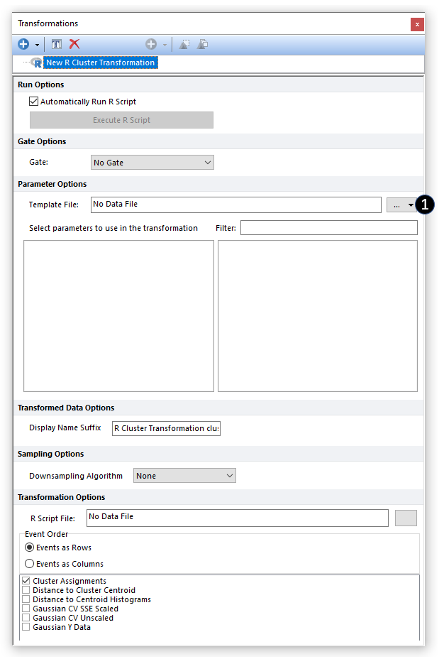
Figure 9.126 The transformation windows populated with a New R Cluster Transformation.
The Transformation window will be populated with the parameters contained in the selected *.FCS file.
5. Select the parameters that will be included in the mat matrix (Figure below - Step 2). Parameters can be filtered or sorted to assist in the selection of parameters when multiple parameters are available in the template file.
6. Select or change to the appropriate Parameter Scaling Options for each of the selected parameters if required (a scale of interest can be applied to All or Checked parameters) (Figure below - Step 3).
7. (Optional) Select a gate from the Gate drop down menu to only include the events within that gate in the mat matrix (Figure below - Step 4).
8. (Optional) The user can customize the Display Name Suffix for the k-means transformation by entering information into the adjacent text box. This modifies what is displayed on a plot when the transformation is applied.(Figure below - Step 5)
9. (Optional) Select a Sampling Option (Figure below - Step 6). Although multiple Sampling Methods are available (please refer to the Sampling Options chapter for more details), the default Downsampling Algorithm for an R Cluster Transformation transformation is None, thus all available events (i.e. the ones defined with the Gate drop-down menu) will be used.
10. Click on the ellipsis at the right of the R Script File field to browse for an R script file (Figure below - Step 7).
11. Select the Event Order. This option define the orientation of the mat matrix. If Events as Row is selected, the mat object will have events in rows and parameters in columns. If Events as Columns is selected, the mat object will have events as column and parameters as rows (Figure below - Step 8).
12. Set the output parameters for the clustering (Figure below - Step 9). Here are reported the available cluster output format.
oCluster Assignment: An internal label indicating the cluster membership assigned to each event. This label is internally used by FCS Express for heatmap representation of clusters but it is also accessible through a Data grid.
oDistance to Cluster Centroid: The distance of a given event to the centroid of its cluster. Values are plotted as unique histogram.
oDistance to centroid Histograms: The same as the Distance to Cluster Centroid but in this case values are grouped, and thus plotted, separately for each cluster. Clusters are numbered from 1 to Number of Clusters.
oGaussian CV SSE Scaled: In this representation each event is plotted based on its cluster membership, thus clusters appear as separated histograms. Given that cluster membership is an integer value that goes from 0 to Number of Clusters-1, an artificial noise is introduced to spread out the data. Gaussian SSE scaled means that the standard deviation of the Gaussian (normal distribution) used to represent each cluster is proportional to the Sum of Squared Error of the cluster.
oGaussian CV Unscaled: In this representation each event is plotted based on its cluster membership, thus clusters appear as separated histograms. Given that cluster membership is an integer value that goes from 0 to Number of Clusters-1, an artificial noise is introduced to spread out the data. Gaussian CV unscaled means that the standard deviation of the Gaussian (normal distribution) used to represent each cluster is the same among clusters.
oGaussian Y Data: Events are plotted following a Gaussian (normal distribution).
The result of the steps above will be the following (Figure 9.128):
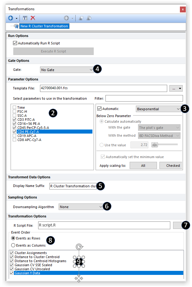
Figure 9.127 The transformation window with a fully set New R Cluster Transformation.
The custom R Cluster Transformation transformation is now ready to be applied to plots.
The R Script will be automatically run when it is applied to a Heat Map or a data grid, or when one of the option in the Transformation dialog are modified. To defer running the R Script, uncheck the box for Automatically Run R Script. Doing so will present you with the button to Execute R Script (Figure 9.129) which can be pressed to calculate on demand.
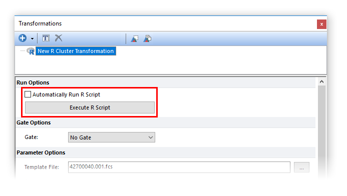
Figure 9.128 Unchecking the Automatically Run R Script box will allow the user to run the R script manually only when required.
Once an R Cluster Transformation transformation has been created, results can be accessed through Heat Maps and Data Grids. The R transformation must be applied to the plots.
R Transformation may be applied to Heat Maps and Data grids by any of the following methods:
Drag and Drop (Figure 9.130)
1. Left click and hold on New R Cluster Transformation from the Transformation window.
2. Drag the transformation to the intended object (Heat Map or Data Grid).
3. Release the mouse button.
The R transformation will be applied to the object. If the object is an Heat Map plot, the title of the plot will now include the text "R Cluster Transformation clustered" to indicate the transformation has been applied.
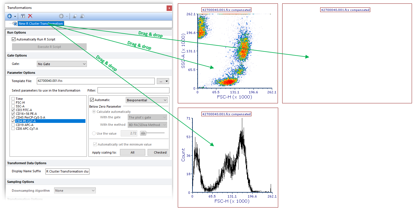
Figure 9.129 Applying an R Cluster Transformation to a plot by dragging the transformation from the Transformation navigator to the plot (green arrow).
Using Transformation Window Commands
•R Cluster may be applied to individual or multiple plots by performing either option outlined in red in the Transformations window below (Figure 9.131).

Figure 9.130 Commands to Apply Transformation to Plot(s)
•Right-click the name of the R cluster and click Apply to selected plot or Apply to all plots button in pop up menu (Figure 9.132).
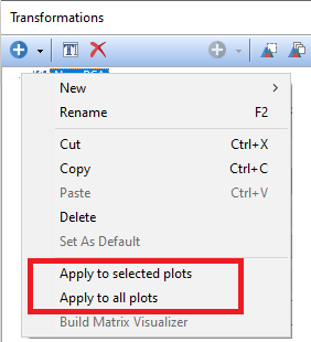
Figure 9.131 Commands to Apply Transformation to Plot(s)
Using the Formatting Dialog (Figure 9.133)
1. Access the Overlays formatting dialog (for 1D plots, 2D plots and Heat map) or the Formatting→General dialog (for Data Grids).
2. Choose the R Cluster Transformation to apply from the Transformation drop down.
3. Click OK.

Figure 9.132 Applying an R Cluster Transformation to a plot by selecting the R Cluster transformation from the Transformation dropdown of the Formatting Overlays dialog.
The result of the previous methods for 2D plot, Heat Map and 1D plot is represented in Figure 9.134. When an R Cluster Transformation has been applied to a 2D plot, Heat Map or 1D plot, the suffix "R Cluster Transformation clustered" will appear in the plot title.

Figure 9.133 The heatmap title contains the "R Cluster Transformation clustered" siffix when an R Cluster Transformation is applied.
2D plots, 1D plots and heatmap can now be used to create gates, markers and well gates suitable for downstream analysis (please refer to the Heat Map section of the Working with k-means parameter chapter for more info on how to create well gates) (Figure 9.135).

Figure 9.134 Examples of 1D Gate ("Cluster 1" gate on the left), rectangle 2D Gate ("Cluster 2" gate on the left), Well Gate (blue well gate in the Heat map) and Marker (M1 marker on the right).
