Scatter with Regression Plots
To insert a Scatter with Regression plot,
| 1. | Select the Insert→2D Plots→Scatter with Regression command (Figure 11.39). |

Fig. 11.36 Inserting a scatter with regression plot.
| 2. | Click (or click-drag) on your layout where you want the plot to appear. |
Note: The plot will appear showing data from the top Custom Data grid, i.e., the Custom Data grid which was most recently selected or edited. The top Custom Data grid is the one most recently accessed. If more than one Custom Data grid exists in your layout, you may choose which Custom Data grid the Scatter with Regression plot refers to from the Active Files tab of the Select a Data File dialog which appears when changing the current data file.
| 3. | Change the X- and Y-axes to the desired parameters. |
To Format a Scatter with Regression Plot:
| 1. | Right click on the plot. |
| 2. | Choose Format to access plot formatting options. |
| 3. | Choose the Regression fit category. |
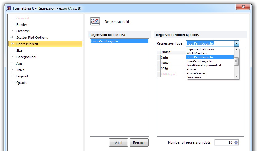
In the regression fit category you may choose the Regression Type (Figure 11.40) from the drop down list of available regression curve equations to best fit your data.

Fig. 11.37 Formatting a scatter with regression plot.
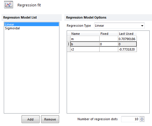
Note that multiple fits may be added or removed by using the Add and Remove buttons under the Regression Model List. The Regression Model Options also allow you to see the model parameters and enter a fixed parameter where applicable (Figure 11.41). The model parameters may later be added to a layout as a live updating token via Scatter with Regression Tokens.
You may also increase the Number of regression dots to give the curve a smoother appearance.

Fig. 11.38 Regression Model Options with a Linear and Sigmoidal fit added to the Regression Model List for comparison. Parameters for the regression model are displayed on the right and a fixed parameter may be typed in the Fixed column. Note in the example that the line was forced through zero by adding a fixed value of "0" to the column.
