Autofit Selection (1 Cycle Analysis)
Setting gates to exclude doublets:
In order to exclude doublets, we will examine a 2D dot plot of the DNA fluorescence height versus the DNA fluorescence area signal and draw a gate on the single cell events. Many times, users will also use the plot of the DNA fluorescence width signal versus the DNA fluorescence area signal. The Height signal corresponds to the peak intensity of fluorescence pulse from the DNA dye. The Area signal is the calculated area under the fluorescence pulse emitted by the DNA dye. The Width signal represents the length of time of the fluorescence pulse emitted by the DNA dye. The specific geometry of the laser beam and other instrument factors determine which parameters are best suited to discriminate single cell events from doublets. In our example, DNA fluorescence area signal is the FL2-A parameter, DNA fluorescence width is the FL2-W parameter, and DNA fluorescence height is the FL2-H parameter.
If a new blank layout is already open then proceed to step 2.
1.Select the File tab→New→New.
2.Select the Insert tab→2D Plots→Dot command.
3.Click anywhere inside the blank layout.
The Select a Data File dialog appears (Figure T19.1).
4.Navigate to the Tutorial Sample Data folder.
5.Make sure that FCS files (*.*, *.fcs, *.lmd) is chosen as the Files of type.
6.Select the file BD.LMD.FCS (Figure T19.1).
7.Click Open.
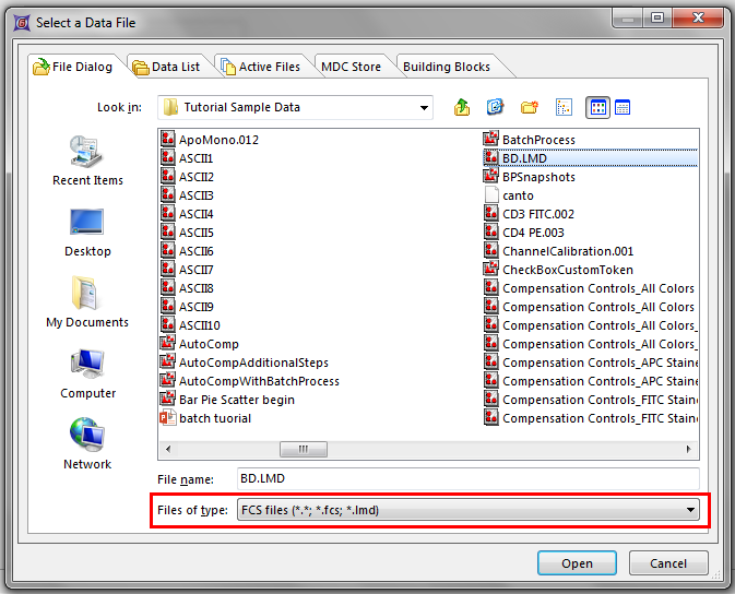
Figure T19.1 Select a Data File Dialog
A dot plot appears on the layout
7.Left-click on the x-axis and select FL2-H from the pop-up menu.
8.Left-click on the y-axis and select FL2-A from the pop-up parameter menu. The dot plot should appear similar to Figure T19.2.
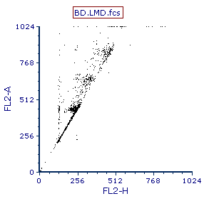
Figure T19.2 Dot Plot of FL2-H vs FL2-A
We will now create a gate on the 2D plot to exclude the doublets as well as to exclude what appear to be tetraploid amounts of DNA. We are excluding these cells with higher amounts of DNA because we want to perform a single cycle DNA analysis. Please refer to Figure T19.3 during the following steps. For more information on creating gates, please refer to the Gating tutorial.
9. Select the Gating tab →Create Gates→Polygon command.
10. Create a polygon gate similar to the gate shown in Figure T19.3.
The Create a New Gate dialog appears.
12. Name the gate 'singlets HA'.
The gate should look similar to Figure T19.3.
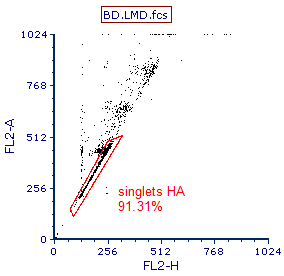
Figure T19.3 Gate to Exclude Doublets and Cells iwth High DNA Content
We are now ready to use the Autofit function in MultiCycle to perform a DNA cell cycle analysis.
Inserting a MultiCycle histogram:
13. Select the Insert tab→1D Plots→MultiCycle DNA command (Figure T19.4).
14. Click on a blank area of the layout.

Figure T19.4 Selecting the Insert Muticycle DNA Command
The Select DNA parameter dialog appears, as shown in Figure T19.5. Please refer to Figure T19.5 for the following steps.
18. Select FL2-A as the Parameter, shown highlighted in blue.
19. Click OK.
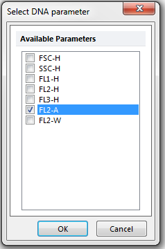
Figure T19.5 Select DNA Parameter Dialog
The histogram of FL2-A, gated on singlets HA, is analyzed by MultiCycle using the Autofit function and appears on the layout (Figure T19.6). Note that your plot may differ from the figure depending on your singlets gate shape.
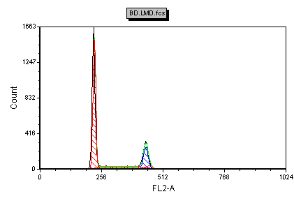
Figure T19.6 MultiCycle Analysis of FL2-A Using Singlets HA Gate
We will now zoom into the region of interest on the Multicycle plot to improve the fit.
20. Right-click on the Multicycle plot and select Magnify (Resolution) from the pop-up menu.
21. Drag the cursor, which is now a crosshair, around the region of interest as shown (Fig. T 19.7, left).
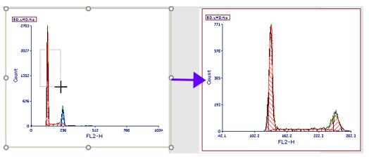
Figure T19.7 Magnifying resolution on a MultiCycle plot to improve the fit of the model
22. Release the cursor. The Multicycle plot's fit has updated, and only one cycling population is now detected, depicted in red (Fig. T 19.7, rright).
We will now display the legend information associated with the MultiCycle DNA analysis.
21. Right-click on the histogram to bring up the associated pop-up menu.
22. Select Format from the pop-up menu.
23. Select Legend from the categories section of the Formatting dialog (Figure T19.8).
24. Click on the Visible checkbox.
25. Click OK (Figure T19.8).
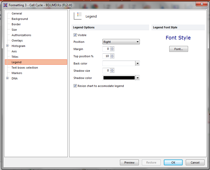
Figure T19.8 Formatting the DNA histogram to Display the Legend Associated with MultiCycle Analysis
Alternatively, the histogram legend information can be displayed using the Format Legend command, as follows:
•Left-click to select the histogram; it should be outlined in green.
Select the Format→Plot Options→Legend command (Figure T19.9).

Figure T19.9 Selecting the Format Legend Command
The Formatting Legend dialog appears (Figure T19.10).
•Click on the Visible checkbox in the Formatting Legend dialog.
•Click OK.
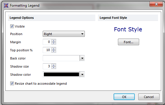
Figure T19.10 Formatting Legend Dialog
The legend associated with the MultiCycle DNA analysis will appear to the right of the histogram (Figure T19.11).
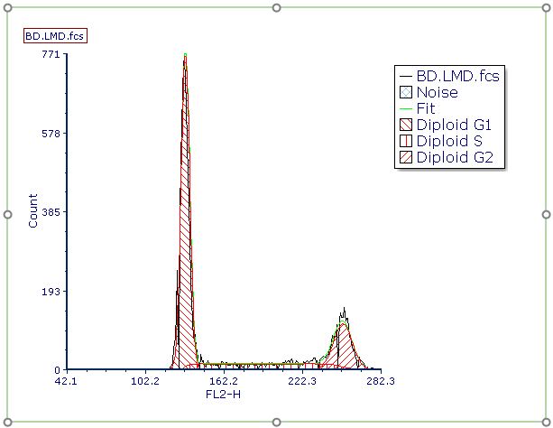
Figure T19.11 MultiCycle DNA Histogram Cell Cycle Analysis with Associated Legend
As you can see from the legend, this histogram contains only diploid cells and therefore a single cycle analysis was performed by the Autofit function of MultiCycle. We can confirm this by examining the MultiCycle information on the ribbon.
26. Left-click to select the histogram, it should be outlined in green (Figure T19.11).
27. Select the MultiCycle tab (Figure T19.12).

Figure T19.12 The Multicycle Tab
Notice that Autofit and Model 1 are highlighted in grey (Figure T19.12). This indicates that the MultiCycle Autofit function and that Model 1 are being used to analyze this DNA histogram. Also notice that 1 Cycle, indicated by the cursor in Figure T19.11, was used in the analysis.
Note: For an explanation of the differences between all the models, please see the De Novo Software DNA/Multicycle AV knowledgebase page.
We will now view all the different statistics for the DNA analysis of this histogram.
28. Right-click on the DNA histogram to bring up the associated pop-up menu.
29. Select Statistics→DNA Cycle Statistics from the pop-up menu (Figure T19.13).
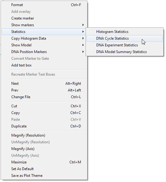
Figure T19.13 DNA Cycle Statistics Pop-up Menu Item
The DNA Cycle Statistics window of the current model (Model 1) will now appear (Figure T19.14). Note that you will have slightly different values for the statistics depending on how your singlet gate was drawn.
30. Move the DNA Cycle Statistics window beneath the plot (Figure T19.14).
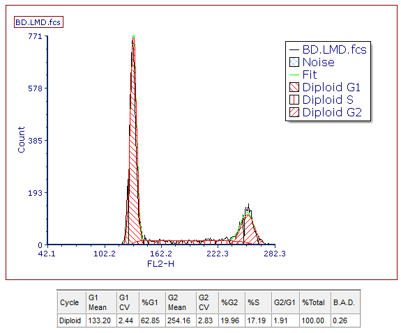
Figure T19.14 DNA Cell Cycle Statistics from the MultiCycle Model 1 Analysis of the Histogram
31. Right-click on the DNA Histogram to bring up the associated pop-up menu.
32. Select Statistics→DNA Model Summary Statistics from the pop-up menu, previously shown in Figure T19.13.
The DNA Model Summary Statistics window, showing all of the six defined MultiCycle models applied to the current histogram, appears. The six models shown in the DNA Model Summary Statistics window correlate respectively with the six models shown in the MultiCycle→Model to Display group (Figure T19.12). The DNA Model Summary Statistics displays the default statistics set in FCS Express preferences which we will change later in the tutorial.
33. Move the DNA Model Summary Statistics window under the DNA Cell Cycle Statistics window (Figure T19.15).
34. Right-click on the DNA Histogram to bring up the associated pop-up menu.
35. Select Statistics→DNA Experiment Statistics from the pop-up menu, previously shown in Figure T19.13.
The DNA Experiment Statistics window with the interpretation of the DNA model and the experiment statistics will appear.
36. Move the DNA Experiment Statistics window next to the DNA Model Summary Statistics window (Figure T19.15).
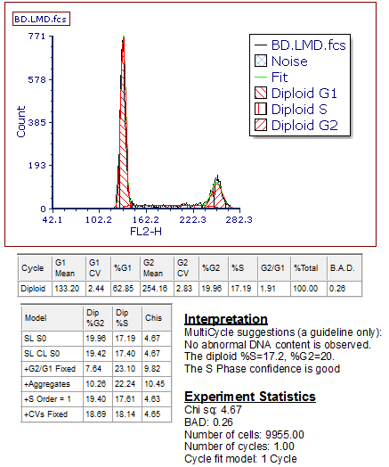
Figure T19.15 DNA Histogram with All of the MultiCycle Statistics Windows
In the next section, we will perform an expanded analysis with Autofit.
