Clustering

Step

Description

Batch Self-Organizing Map

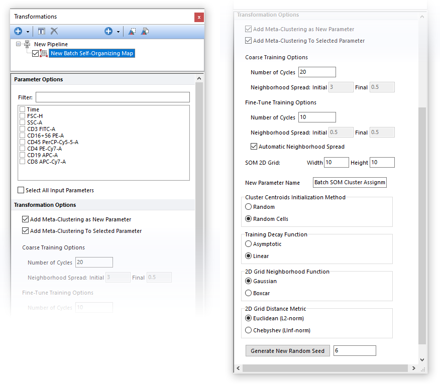
The Batch Self-Organizing Map step performs Batch SOM clustering on the input population, using parameters selected in the Parameter Options list (see image below). Parameters can be filtered or sorted to assist in the selection of parameters when multiple parameters are available in the template file. Using the Filter: field a user can remove unwanted parameters from view to simplify selection.  For example, if a user only wanted to select area parameters typing "-A" in the field would reduce the number of parameters seen in the parameter list. By right clicking in the parameters section, you can use Sort Ascending, Sort Descending, or Unsorted to easily manage parameter ordering and facilitate parameter selection.  In the right click menu, you can easily select parameters by utilizing Check All, Uncheck All, Check Selected, Uncheck Selected, Invert Selection on All.  The options Check Selected and Uncheck Selected allow for using the shift key or Ctrl key to multi-select parameters and check or uncheck them all simultaneously.

The output of the Batch SOM (Batch Self-Organizing Map) step is a list of Cluster Assignment, which is an internal label indicating the SOM node membership that is automatically assigned to each event. The cluster assignment can be displayed by the user on 1D plots, 2D plots, Plate Heatmap plots, and Data Grid.

The output parameter of the Batch SOM pipeline step can be used as input parameter for the Minimum Spanning Tree pipeline step.

Once the Batch SOM clustering is displayed on the Plate Heat Map, the following actions can be performed on the Plate Heat Map:

•Modify the well size

•Have well size dependent on a statistic such as number of events in the node

•Set the Parameter and Statistic for display

•Change the Color Level and Color Scheme

•Create Well gates to select one or more clusters (i.e. wells) and use those gates/clusters for downstream analysis.

Some background on Batch Self-Organizing Map (i.e. Batch SOM) can be found below.

Batch SOM is a variation of the original SOM algorithm (please refer to the SOM section for more details on Self-Organizing Maps) with the following advantages:

•In the Batch SOM there is no Learning Rate function so the number of required parameters is reduced.

•The Batch SOM algorithm converges faster than the stepwise "gradient" method.

•The Batch SOM algorithms is faster than the SOM algorithm since it can run using all the cores in the computer.

The main difference between the classical SOM and the Batch SOM is in the way the 2D grid is trained. With classical SOM, the 2D Grid is trained and updated one data point at a time (i.e. one data point at every iteration), while in the Batch SOM, the 2D Grid is trained using the entire dataset as a single iteration then updating the 2D Grid. With every iteration, the Winner node (also called Best Matching Unit, or "BMU") is calculated for every data point of the dataset, not just for a single randomly-selected data point.

That means that in every iteration and for every node, the set of data points that have that node as their BMU is known.

With the Neighborhood function (please refer to the SOM section for more details ), the set of data points referring to each neighborhood can also be defined (i.e. all the data points whose BMU is a node of the neighborhood).

In the Weight Updating phase, the location of each SOM node in the high dimensional space is updated so that each node moves towards the center of all the points referring to its neighborhood. The location is calculated as the cumulative contribution of each data points properly weighted on the high dimensional location using the neighborhood distance between the node of interest and their BMU.

The training of the 2D Grid is performed by repeating the procedure above several times in two subsequent training phases.

The two training phases are:

1.Coarse training phase. During this phase, the neighborhood spread decreases (see the Training Decay Function option below) from an initial value to a final value. The number of cycle, and both the Initial and Final Neighborhood Spreads values for this phase, can be defined by the user via the Coarse Training Options fields (see image below). Note that by default the Initial and Final Neighborhood Spreads values are automatically calculated.

2.Fine-Tune training phase. During this phase the neighborhood spread decreases (see the Training Decay Function option below) from an initial value to a final value. The initial value of the neighborhood spread can not exceed the final value of the neighborhood spread of the coarse phase (as a recommendation, the default initial value of the neighborhood spread for this phase should match the final value of the neighborhood spread of the coarse phase). Also, the final value of the neighborhood spread in this phase cannot be less then half of its initial value in this phase (as a recommendation, the neighborhood spread value in this phase should be held constant). The number of cycles, and both the Initial and Final Neighborhood Spreads values for this phase, can be defined by the user via the Fine-Tune Training Options fields (see image below). Note that by default the Initial and Final Neighborhood Spreads values are automatically calculated.

The output of the Batch SOM step is a list of Cluster Assignment, which is an internal label indicating the SOM node membership that is automatically assigned to each event. The cluster assignment can be displayed by the user on 1D plots, 2D plots, Plate Heat Map plots, and Data Grid.

The high-dimensional locations of the nodes can be used as Input parameter for the Minimum Spanning Tree pipeline step.

The name of the new parameter created by the Batch SOM algorithm can also be customized by the user via the "New Parameter Name" field.

The Batch SOM algorithm is stochastic. To make it reproducible, a fixed Seed may be set. If the same dataset and the settings are used, by retaining the same Random Seed value, the same result will be achieved. SOM may be run multiple times with different Random Seeds to evaluate the stability and the consistency of the result.

Once the Batch SOM clustering is displayed on the Plate Heat Map, the following actions can be performed on the Plate Heat Map:

•Modify the well size

•Have well size dependent on a statistic such as number of events in the node

•Set the Parameter and Statistic for display

•Change the Color Level and Color Scheme

•Create Well gates to select one or more clusters (i.e. wells) and use those gates/clusters for downstream analysis. Meta-clusters may also be automatically gated using Heat Map Well Gates

Louvain Communities

The Louvain method for community detection is a method to extract communities from large networks created by Blondel et al. from the University of Louvain in 2008.

The input dataset is represented by a weighted network of data points (i.e. cells) in which each data point is connected with its closest neighbor by a weighted edge. In this representation, communities (i.e. phenotypically-similar cells), are expected to manifest as groups of highly-interconnected nodes. In the Louvain method, communities are indeed defined by maximizing the local modularity, which is a parameter that measures the relative density of connections inside communities with respect to connections outside communities.

The process is formally executed in 3 different steps:

1) Local move phase

Each node in the network is assigned to its own community. Then, given a node i of the network, the change in modularity is calculated for removing i from its own community and moving it into the community of each neighbor j of i. Once all the neighbors j have been tested, node i is moved to the community j that ensure the largest increase in modularity. If none of the moves increases modularity, node i is not moved to any community.

To speed up the calculation, the process described above is not repeated for each node of the network, but just for a subset of them. The list of revisited nodes is indeed “pruned” from the entire network to a much smaller group of nodes that have a high potential to actually swap communities. This approach is called “Louvain pruning”.

The Local move phase stops when it is no longer possible to increase the local modularity by performing a node move. 

2) Aggregation phase

Each community found in Step 1 is grouped into one super-node to create a weighted network of super-nodes.

3) Repeat

The process restarts, with Step 1 being run on the network of super-nodes generated in Step 2. The entire process repeats until no increase in local modularity is gained.

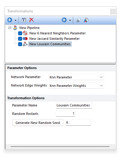
The Louvain algorithm is a greedy heuristic algorithm. Solving the community assignments that maximize the overall modularity is computationally infeasible. The Louvain method acknowledges this and attempts to find the best "local solution". It does this by randomly selecting a path through the network in Step 1 above. The random path impacts the final results because each time a node moves, the local modularity profile changes accordingly. This, in turn, influences the neighbor's decision to merge. For this reason, the overall calculation (Steps 1-2-3) can be executed more than once, with a different random start each time. The number of time the whole process should restart is defined by the user with the Random Restarts option (see picture below). 5 restarts is usually a good value to try. The best results are then chosen using the final modularity score. The community assignments with the highest overall modularity score are selected.

To make the process reproducible, a fixed Seed may be set. If the same dataset and the settings are used, by retaining the same Random Seed value, the same result will be achieved. The Louvain Community pipeline step may be run multiple times with different Random Seeds to evaluate the stability and the consistency of the result.

Other notes to consider:

•Convergence of the Louvain algorithm is guaranteed. 

•The first iteration of the Louvain algorithm (i.e. the first time Steps 1 and 2 are executed) takes the majority of the execution time. However, FCS Express vastly speeds up this part by using the “Louvain pruning” technique.

•Even very large networks tend to converge in less than 10 overall iterations. This is because the network “shrinks” with each iteration, so there are fewer nodes to visit for moving.

The output of the Louvain Community pipeline step is a new parameter called Louvain Communities defining the community assignment for each cell of the input dataset. The "Louvain Communities" parameter can be plotted on Histograms, 2D plots and Plate Heat Map. We suggest using Plate Heat Maps, since it allows the following actions:

•Modification of the well size

•Well size dependent on a statistic such as number of events in the node

•Set the Parameter and Statistic for display

•Change the Color Level and Color Scheme

•Create Well gates to select one or more clusters (i.e. wells) and use those gates/clusters for downstream analysis.

Consensus Clustering

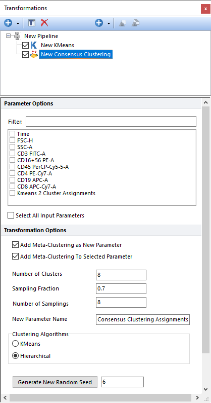
Performs Consensus Clustering, on the input population, using the parameters selected in the Parameter Options list (see image below). Parameters can be filtered or sorted to assist in the selection of parameters when multiple parameters are available in the template file. Using the Filter: field a user can remove unwanted parameters from view to simplify selection.  For example, if a user only wanted to select area parameters typing "-A" in the field would reduce the number of parameters seen in the parameter list. By right clicking in the parameters section, you can use Sort Ascending, Sort Descending, or Unsorted to easily manage parameter ordering and facilitate parameter selection.  In the right click menu, you can easily select parameters by utilizing Check All, Uncheck All, Check Selected, Uncheck Selected, Invert Selection on All.  The options Check Selected and Uncheck Selected allow for using the shift key or Ctrl key to multi-select parameters and check or uncheck them all simultaneously.

Consensus clustering is a technique to find a single clustering result (i.e. a consensus) when many clustering runs are performed.

Consensus clustering in FCS Express is performed with the Monti method (Monti et al. Consensus Clustering: A Resampling-Based Method for Class Discovery and Visualization of Gene Expression Microarray Data. Machine Learning. 52. 91-118. 10.1023/A:1023949509487). Briefly, subsets of points are sampled from the input dataset and clustering is performed on each subset. A pairwise consensus matrix is then created to calculate the frequency with which every pair of points are found in the same cluster. The consensus matrix (M) can then be converted to be a distance/dissimilarity matrix (1-M) and further used to perform a final clustering step, which finally give the consensus clustering.

This clustering approach is quite computationally heavy, the highest number of objects that can be clustered is set to 8000. So, the Consensus Clustering step is suitable to cluster clusters generated by other clustering steps (which number is usually lower than 8000). This procedure is also called Meta-clustering.

The output of the Consensus Clustering step is a list of Cluster Assignment, which is an internal label indicating the cluster membership that is automatically assigned to each event. The cluster assignment can be displayed by the user on 1D plots, 2D plots, Plate Heatmap plots, and Data Grid.

The Cluster Assignment can be used as Input parameter for the Minimum Spanning Tree pipeline step.

When the input parameter is a cluster assignment (common occurrence with this type of clustering; see comment above), the current clustering steps performs a meta-clustering. In this case, the following options are particularly useful:

•Add Meta-Clustering as New Parameter. By checking this check box, the meta-cluster assignment generated by this clustering step can be added as new parameter and thus be displayed on 1D plots, 2D plots, Plate Heatmap plots, and Data Grids.

•Add Meta-Clustering to Selected Parameter. By checking this check box, the meta-cluster assignment generated by this clustering step can be visualized as a colored border around nodes, when the input parameter is displayed on a Heatmap plot.

The following settings may also be customized by the user:

•Number of Clusters. This defines the number of clusters which should be found.

•Sampling Percentage. This defines the fraction of events sampled at every repetition.

•Number of Samplings. This defines the number of repetition.

•New Parameter Name. The name of the new parameter (i.e. the one containing the cluster assignment for each input data) can be specified in this field.

•Clustering Algorithm. This option allows a user to define whether the consensus clustering should be performed using k-Means or Hierarchical clustering.

•Generate New Random Seed. Setting a Seed allows to ensure reproducibility with algorithms that rely on random initialization. Changing the Seed is a good way to evaluate the impact of randomness on the clustering result.

Once the Consensus clustering is displayed on the Heat Map, the following actions can be performed on the Heat Map:

•Modify the well size

•Have well size dependent on a statistic such as number of events in the node

•Set the Parameter and Statistic for display

•Change the Color Level and Color Scheme

•Create Well gates to select one or more clusters (i.e. wells) and use those gates/clusters for downstream analysis.

Hierarchical Clustering

Performs Single-linkage agglomerative clustering, on the input population, using the parameter(s) selected in the Parameter Options list (see image below). Parameters can be filtered or sorted to assist in the selection of parameters when multiple parameters are available in the template file. Using the Filter: field a user can remove unwanted parameters from view to simplify selection.  For example, if a user only wanted to select area parameters typing "-A" in the field would reduce the number of parameters seen in the parameter list. By right clicking in the parameters section, you can use Sort Ascending, Sort Descending, or Unsorted to easily manage parameter ordering and facilitate parameter selection.  In the right click menu, you can easily select parameters by utilizing Check All, Uncheck All, Check Selected, Uncheck Selected, Invert Selection on All.  The options Check Selected and Uncheck Selected allow for using the shift key or Ctrl key to multi-select parameters and check or uncheck them all simultaneously.

This clustering approach is quite computationally heavy, the highest number of objects that can be clustered is set to 8000. So, the Hierarchical Clustering step is suitable to further cluster clusters generated by other clustering steps (which number is usually lower than 8000). This procedure is also called Meta-clustering.

The output of the Hierarchical Clustering step is a list of Cluster Assignment, which is an internal label indicating the cluster membership that is automatically assigned to each event. The cluster assignment can be displayed by the user on 1D plots, 2D plots, Plate Heatmap plots, and Data Grid.

The Cluster Assignment can be used as Input parameter for the Minimum Spanning Tree pipeline step.

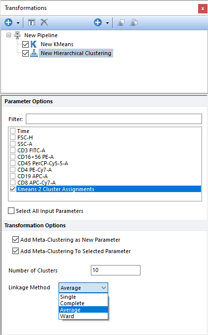
When the input parameter is a cluster assignment (common occurrence with this type of clustering), the current clustering steps perform a meta-clustering. In this case, the following options are particularly useful:

•Add Meta-Clustering as New Parameter. By checking this check box, the meta-cluster assignment generated by this clustering step can be added as new parameter and thus be displayed on 1D plots, 2D plots, Plate Heatmap plots, and Data Grids.

•Add Meta-Clustering to Selected Parameter. By checking this check box, the meta-cluster assignment generated by this clustering step can be visualized as a colored border around nodes, when the input parameter is displayed on a Heatmap plot.

The following settings may also be customized by the user:

•Number of Clusters. Defines the number of clusters to attempt to find.

•Linkage Method. Possible options for linkage are:

oSingle. The distance between two clusters is defined by the smallest distance between a point in the first cluster and a point in the second clusters. Also referred to as the "nearest-neighbor" method.

oComplete. The distance between two clusters is defined by the larger distance between a point in the first cluster and a point in the second clusters. Also referred to as the "furthest-neighbor" method.

oAverage. The distance between two clusters is defined by the average distance between the points in the first cluster and the points in the second cluster.

oWard. The Ward method (also called minimum-variance method) minimizes the within-cluster variance. Two clusters are merged if the variance of the resulting cluster is the smallest variance possible as compared to the variance resulting from merging any other pair of clusters. The Ward method aims at finding compact, spherical clusters.

Once the Hierarchical clustering is displayed on the Heat Map, the following actions can be performed on the Heat Map:

•Modify the well size

•Have well size dependent on a statistic such as number of events in the node

•Set the Parameter and Statistic for display

•Change the Color Level and Color Scheme

•Create Well gates to select one or more clusters (i.e. wells) and use those gates/clusters for downstream analysis.

Kmeans

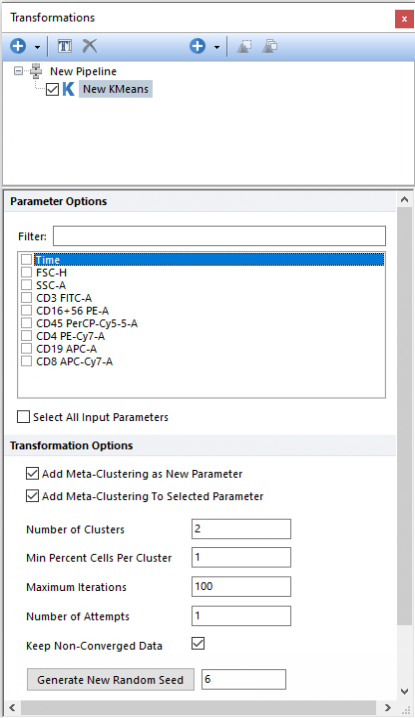
Performs Kmeans clustering, on the input population, using the parameter(s) selected in the Parameter Options list (see image below). Parameters can be filtered or sorted to assist in the selection of parameters when multiple parameters are available in the template file. Using the Filter: field a user can remove unwanted parameters from view to simplify selection.  For example, if a user only wanted to select area parameters typing "-A" in the field would reduce the number of parameters seen in the parameter list. By right clicking in the parameters section, you can use Sort Ascending, Sort Descending, or Unsorted to easily manage parameter ordering and facilitate parameter selection.  In the right click menu, you can easily select parameters by utilizing Check All, Uncheck All, Check Selected, Uncheck Selected, Invert Selection on All.  The options Check Selected and Uncheck Selected allow for using the shift key or Ctrl key to multi-select parameters and check or uncheck them all simultaneously.

The following settings may also be customized by the user (please refer to the Defining a k-Means cluster analysis chapter for more details):

•Number of Clusters

•Min percent Cells Per Cluster

•Maximum Iterations

•Number of Attempts

•Keep-Non-Converged Data

The output of the Kmeans step is a list of Cluster Assignment, which is an internal label indicating the cluster membership that is automatically assigned to each event. The cluster assignment can be displayed by the user on 1D plots, 2D plots, Plate Heatmap plots, and Data Grid.

The Cluster Assignment can be used as Input parameter for the Minimum Spanning Tree pipeline step.

When the input parameter is a cluster assignment, the current clustering steps perform a meta-clustering. In this case, the following options are particularly useful:

•Add Meta-Clustering as New Parameter. By checking this check box, the meta-cluster assignment generated by this clustering step can be added as new parameter and thus be displayed on 1D plots, 2D plots, Plate Heatmap plots and Data Grid.

•Add Meta-Clustering to Selected Parameter. By checking this check box, the meta-cluster assignment generated by this clustering step can be visualized as a colored border around nodes, when the input parameter is displayed on an Heatmap plot.

Finally, the Kmeans algorithm is stochastic. To make it reproducible, a fixed Seed may be set. If the same dataset and the setting are used, by retaining the same Random Seed value, the same result will be achieved. Kmeans may be run multiple times with different Random Seeds to evaluate the stability and the consistency of the result.

Once the k-Means clustering is displayed on the Heat Map, the following actions can be performed on the Heat Map:

•Modify the well size

•Have well size dependent on a statistic such as number of events in the node

•Set the Parameter and Statistic for display

•Change the Color Level and Color Scheme

•Create Well gates to select one or more clusters (i.e. wells) and use those gates/clusters for downstream analysis.

Self-Organizing Map

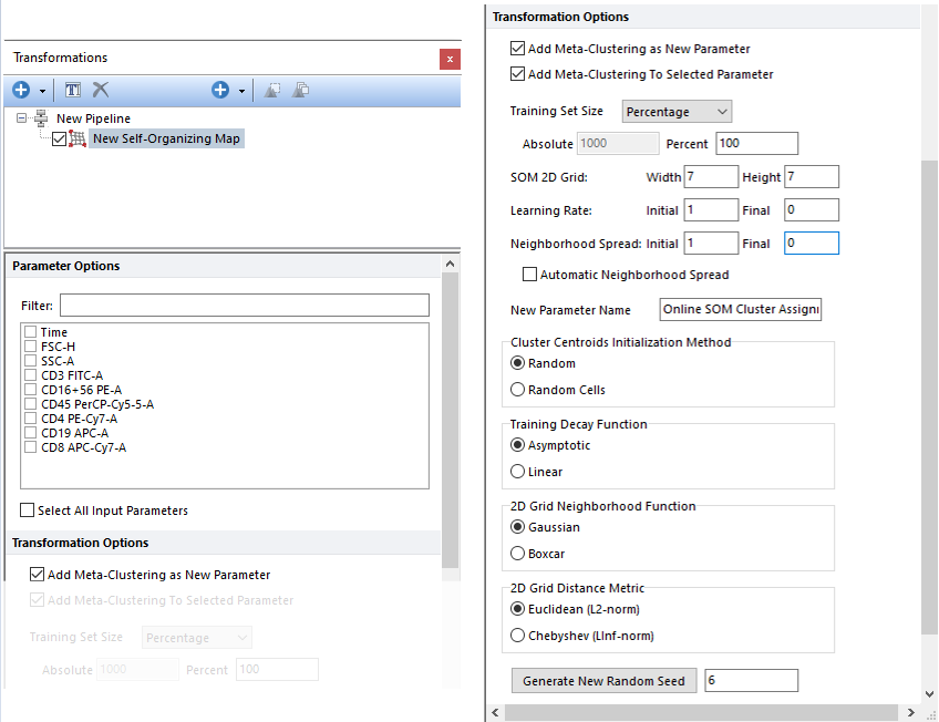
This step performs SOM clustering on the input population, using the parameters selected in the Parameter Options list (see image below). Parameters can be filtered or sorted to assist in the selection of parameters when multiple parameters are available in the template file. Using the Filter: field a user can remove unwanted parameters from view to simplify selection.  For example, if a user only wanted to select area parameters typing "-A" in the field would reduce the number of parameters seen in the parameter list. By right clicking in the parameters section, you can use Sort Ascending, Sort Descending, or Unsorted to easily manage parameter ordering and facilitate parameter selection.  In the right click menu, you can easily select parameters by utilizing Check All, Uncheck All, Check Selected, Uncheck Selected, Invert Selection on All.  The options Check Selected and Uncheck Selected allow for using the shift key or Ctrl key to multi-select parameters and check or uncheck them all simultaneously.

The output of the SOM (Self-Organizing Map) step is a list of Cluster Assignment, which is an internal label indicating the SOM node membership that is automatically assigned to each event. The cluster assignment can be displayed by the user on 1D plots, 2D plots, Plate Heatmap plots, and Data Grid.

The output parameter of the SOM pipeline step can be used as input parameter for the Minimum Spanning Tree pipeline step.

Once the SOM clustering is displayed on the Plate Heat Map, the following actions can be performed on the Plate Heat Map:

•Modify the well size

•Have well size dependent on a statistic such as number of events in the node

•Set the Parameter and Statistic for display

•Change the Color Level and Color Scheme

•Create Well gates to select one or more clusters (i.e. wells) and use those gates/clusters for downstream analysis.

Some background on Self-Organizing Map (i.e. SOM) can be found below, together with a description of all the settings available in FCS Express to customize the SOM calculations.

Self-Organizing Map (i.e. SOM) is a special class of artificial neural networks first introduced by Teuvo Kohonen and is used extensively as a clustering, dimensionality-reduction and visualization tool in exploratory data analysis.

The input and the output data are defined in the same high-dimensional space but the number of output data k (i.e. "nodes" or "neurons") is smaller than the number of input data n. For the sake of simplicity, output nodes can be thought of as centroids in the k-Means clustering and much like k-Means, output nodes for SOM are generally randomly initialized at the initialization of the SOM process.

One of the key points of SOM is that, output nodes also exist in a bi-dimensional space to form a grid in which each node is connected to its neighborhood nodes. The size of the grid is defined by the user (see the Grid Width and the Grid Height options in the image below; the default setting for a standalone SOM step is a 7x7 grid but when the SOM step is added via the FlowSOM pre-defined algorithm, the default setting is a 10x10 grid).

The basic steps of Kohonen’s SOM algorithm can be summarized by the following iterative procedure:

1.Initialization. The location in the high-dimensional space for each of the k output nodes is initialized by picking k random points in high dimensional space. They can be k random locations of the space, generally chosen in a small ‘ball’, or k random points from the input dataset (see the Cluster Centroid Initialization Method in the table below).

2.Sampling. Randomly select a point from the input dataset to present to the SOM nodes.

3.Similarity Matching. Compute the Euclidean distances between the selected point and each SOM node to find the nearest node (i.e. the winner; also called Best Matching Unit, or BMU).

4.Weight Updating. The location of all SOM nodes in the high dimensional space is updated so that nodes move towards the point sampled in Step 2. Each node is updated by a fraction of the current sample point. Said fraction is calculated for each node by a Learning function, which is a function of both the 2D distance to all other nodes and a learning rate(see below). The Learning function is a decreasing function which decreases at every iteration t (see Step 5).

5.Repeat Step 2, 3 and 4 until training is complete .

The Learning function in Step 4 above defines the amplitude of the movement for each node of the 2D grid towards the sample point (i.e. in other words defines how the 2D grid "learns" the shape of the multidimensional dataset). A generalized formula for this function is the following:

Learning = DistHD * α(t) *  h(t)

Where DistHD is the distance, calculated in the high-dimensional space, between the sample point and the node, α(t) is the Learning Rate function and h(t) is the Neighborhood function. Both the Learning Rate and the Neighborhood Functions exist in the range 0 to 1 and are decreasing functions (i.e. they both decrease at every iteration t). Since the Neighborhood function is always equal to 1 for the winner node (see below), the Learning Rate function can be viewed as the as the fraction of the distance covered by the winner node towards the sampled point. For every other nodes, the distance covered towards the sampled points will be equal to, or shorter than that (because of the further penalty caused by h(t), which is based on distance of the nodes to the winner node).

Parameter Options

SOM will be run on the population selected in the main pipeline body, using the parameter(s) selected in the Parameter Options list (see image below). Parameters can be selected individually by clicking on the boxes or by using the right click menu. The right click menu gives the user the option to Select All, Deselect All, or Invert Selection.

Transformation Options

The output of the SOM step is a list of Cluster Assignment, which is an internal label indicating the SOM node membership that is automatically assigned to each event. The cluster assignment can be displayed by the user on 1D plots, 2D plots, Plate Heat Map plots, and Data Grid.

The high-dimensional locations of the nodes can be used as Input parameter for the Minimum Spanning Tree pipeline step.

The name of the new parameter created by the SOM algorithm can also be customized by the user via the "New Parameter Name" field.

The SOM algorithm is stochastic. To make it reproducible, a fixed Seed may be set. If the same dataset and the settings are used, by retaining the same Random Seed value, the same result will be achieved. SOM may be run multiple times with different Random Seeds to evaluate the stability and the consistency of the result.

Once the SOM clustering is displayed on the Plate Heat Map, the following actions can be performed on the Plate Heat Map:

•Modify the well size

•Have well size dependent on a statistic such as number of events in the node

•Set the Parameter and Statistic for display

•Change the Color Level and Color Scheme

•Create Well gates to select one or more clusters (i.e. wells) and use those gates/clusters for downstream analysis. Meta-clusters may also be automatically gated using Heat Map Well Gates