Overlays

Contents
All Spectrum Plots have at least one overlay and a spectrum to display. Additional overlays from the same or different spectral data files can be added in the same way that overlays are added to histograms and other plots in FCS Express. Different gates can also be applied to each overlay, if desired (e.g., Figure 5.56).

Figure 5.56 - Spectral plot with two overlays from different spectral datafiles, each with a different gate applied.
You can add additional overlays by any of the following methods:
•Right-click on the plot and select Add overlay from the pop-up menu. This launches either the Select Data File or the Open Data File dialog depending on the Open Data Dialog user Options; or
•Right-click on the plot and select Add Overlay using Advanced Open Data Dialog (launches the Open Data File dialog), or
•Drag-and-drop file(s) from the Data List onto the plot you wish to overlay, or
•Drag-and-drop a plot from the layout onto the plot you wish to overlay.
The Overlays option controls the spectrum and appearance of spectrum overlays. The selected Overlay to show will be applied to all overlays that are added to a spectrum plot. For example, if Average spectrum is applied to a spectrum plot and a new overlay is added it will also be displayed by showing the average of all events as one line or dot.
You can edit overlays in one of two ways:
•Select the Spectrum plot(s) and use the Format→Plot Options→Overlays command in the ribbon bar.
•Right-click on the Spectrum plot, select Format from the pop-up menu, and choose Overlays from the drop-down at the top of the Formatting dialog (Figure 5.57).

Figure 5.57 - Formatting Spectrum Overlays Dialog
A list of all the overlays on the Spectrum Plot will appear in the list box at the top. You can select one or more overlays using standard Microsoft Windows techniques, including Shift-Click and Ctrl-Click. The properties on the bottom pertain to the currently selected overlay(s). If multiple overlays are selected, the information will appear blank for those properties that are not identical in all selected overlays. If the properties are not blank, then they are identical for all selected overlays. Changing an option will change that property for all selected overlays. For instance, if you select three overlays and change the Gate, the Gate for all three overlays will be modified.
To remove an overlay from a plot, select the overlay(s) and press the Remove button.
To change the order of selected overlay(s) use the up and down arrows (![]() ). The in the legend will authentically update accordingly.
). The in the legend will authentically update accordingly.
Overlay formatting options for Spectrum plots are explained in the table below; additional options specific to Spectrum Plots, which can greatly aid in analysis and report generation, are explained in detail in the Spectrum Plot Specific Options chapter.
Option |
Explanation |
|---|---|
Spectrum |
Change the laser line displayed on the spectrum plot. |
Gate |
If gates are defined, select the gate that will be used to limit the data that is displayed for each Overlay on the spectrum plot. |
Overlay to show |
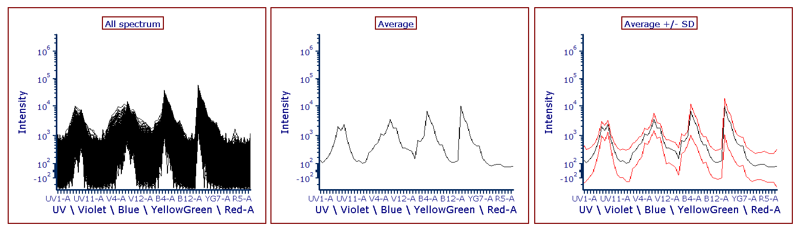
Three choices are available: •All spectrums shows each event as an individual line or dot (left plot below); •Median spectrum shows the median of all events as one line or dot; •Average spectrum shows the average of all events as one line or dot (plot in the middle below);
When either Median spectrum or Average spectrum is selected, the Standard Deviation can also be displayed by checking the Show Std Dev check box (see the Show Std Dev option below). The Standard Deviation is plotted as a dot or line above and below the Median (or the Average). The right plot below shows an example of spectrum plot displaying the Average Spectrum and the Standard Deviation lines. The color of the Std Dev dots/lines can be customized through the Standard Deviation Color drop-down menu (see the Standard Deviation Color option below).
|
Compensation |
If compensation definitions are set, select the definition to use when compensating the data in the overlay. |
Transformation |
If transformations are set, select the transformation to use for each overlay. |
Legend Text |
The text that will appear in the legend beside the symbol for the overlay. Free text can be inserted. If this field is blank the file name of the overlay will appear. A dropdown menu with additional pre-customized legend content is accessible by pressing the ellipsis button next to the legend text. Possible choices are: oKeyword. This can be used to insert keywords from the header of the data file. oGate. This can be used to display the current gate applied to the overlay. oTube Number. This can be used to display the Tube Number of the overlay when a Panel is active. oTube Name. This can be used to display the Tube Name of the overlay when a Panel is active. The above mentioned Legend options apply only to Dot Plots, Color Dot Plots, Histograms and Spectrum Plots. |
Smoothing |
Set the degree of smoothing for the overlay. |
Change data file during Next/Prev/Batch |
If this option is checked, the data file for this overlay will change when doing batch processing, or selecting Previous File or Next File. This option is usually only disabled for a control spectrum, where you have multiple overlays, and want the control to stay the same all of the time. |
Show Std Dev |
When this option is checked, the Standard Deviation is plotted as a dot or line above and below the Average (this option is only available when Average is selected as Overlay to Show, see above). The color of the Std Dev dots/lines can be customized through the Standard Deviation Color drop down menu. |
Visible |
You can hide overlays on a spectrum plot without removing them. Select the overlay file from the list and uncheck Visible. Check Visible to show the overlay again. |
Below are some example of Spectrum plot customizations.
Figure 5.58 shows a Spectrum plot with two Overlays as an Average (see the Overlay to show option in the table above). Please note that a legend is also displayed.

Figure 5.58 Example of Spectrum plot customizations.
Figure 5.59 displays a Spectrum Plot with the Display Mode option set to Color on Density (see Spectrum Plot Specific Options)

Figure 5.59 Example of Spectrum plot customizations.