Adding Merged Files to the Data List

Contents
Cytometry data files are typically added as separate data files in the data list. However, multiple files may be merged together (concatenated) and loaded as a new file using the Merge FCS Files file format from the file of type drop down. Once a merged data file is added to the data list it may be used in any of the plots and analysis your perform in FCS Express. Identifiers for Merged FCS files are controlled via instrument specific settings and may be set as numeric values (file identifiers) or textual (classification identifiers).
Merging data files using the Merge FCS Files file of type is a convenient way to load and visualize multiple files on one plot, for instance, with an antibody titration or drug treatment series, and may prove particularly useful when performing transformations where an algorithm must be run on a file that is representative of all samples in the experiment. Merged files may also be represented in a plate heat map even if they were not acquired on a plate. When using the Merge FCS Files option there is no need to export as a new data file as the files that are selected will be "virtually" merge on the fly. Virtually merged files can be used as any other .FCS File would be used. They can be displayed in any plot types and statistics can be derived from them as well.
Please also see the chapter on Exporting FCS File Data from Multiple Files if you would like to merge multiple data files and save the resulting merged data file as a new .FCS file.
To begin merging data files using the Merge FCS Files option:
1. Open the Data list.
2. Click on the ![]() button.
button.
The Standard Open Data Dialog will appear as in Figure 6.7 below.
Note: based on your User Options, the Advanced Open Data Dialog may appear. If the Advanced Open Data dialog appears, please select the ![]() button to access the Standard Open Data Dialog.
button to access the Standard Open Data Dialog.
3. Click on the Options button at the bottom left of the Select Data File dialog to reveal the Enable drop-down menu.
4. Expand the Enable drop-down menu and select Merge FCS Files (*.fcs, *lmd)
5. Select multiple files from your computer. This can be done by Cmd-Click or Shift-Click.
6. Click Open.
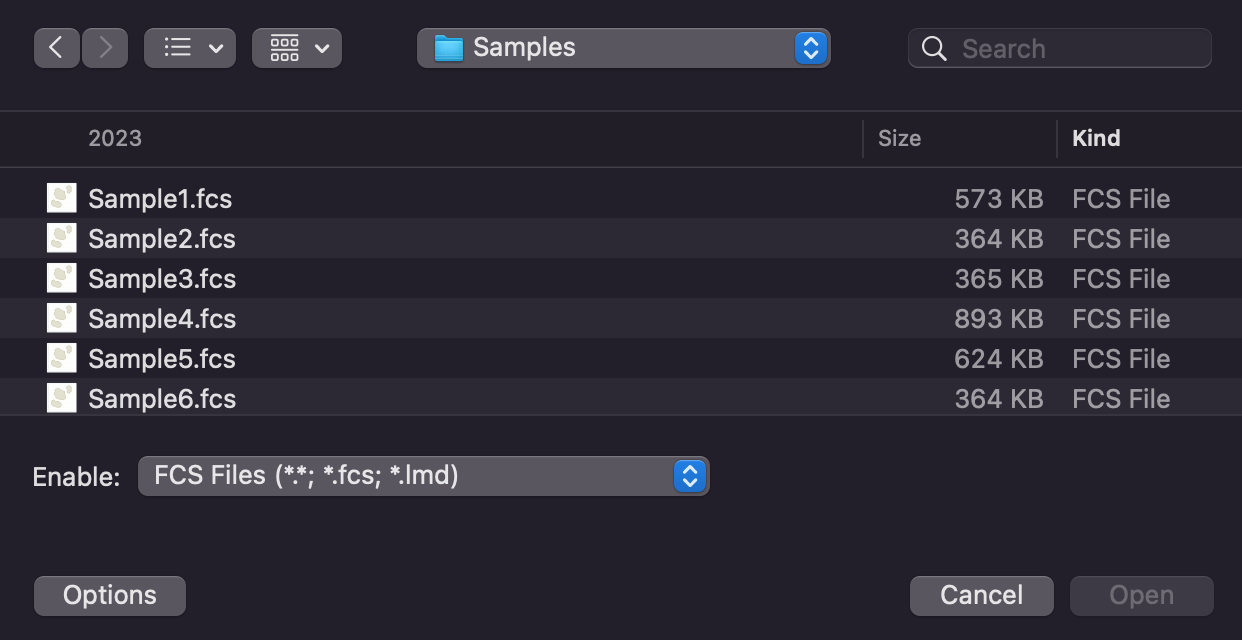

Figure 6. 7 - The Standard Open Data dialog
The selected files will be virtually merged / concatenated in alphabetical order and a single file will be listed for them in the Data List (Figure 6.8).

Figure 6.8 - The Data List with the virtually merged file loaded.
The virtually merged file is concatenated as follow:
•Files are concatenated in alphabetical order.
•The compensation matrix of the first file is applied to all the following files (the compensation matrices of the following files are not used).
•A File Identifier and a Classification File Identifier are added. The first one can be used to discriminate the merged files using 1D and 2D plots afterward. The second one can be used to discriminate merged files using an Plate Heat Map plot afterward.
An example of a virtually merged file is depicted below. The File Identifier parameter can be displayed on 1D and 2D plots. Single files can be selected by Converting and Linking Markers on 1D plots, or by using 1D or regular gates on 2D plots (Figure 6.9, upper panes). The Classification File Identifier parameter can be displayed on 1D and 2D plots. It will display the filename of the individual files within the merged file. Specific files can be identified using markers or gates as described above. The Classification File Identifier can also be displayed in Plate Heat Map plots. With Plate Heat Maps, single files can be selected by using Well Gates (Figure below, lower pane).
, 1D Gates or Well Gates.")
Figure 6.9 - The virtually merged file is loaded into different plots displayin either the File Identifier or the Classificiation File Identifier parameter. Single files are also selected by Markers (Converted and Linked to gates), 1D Gates or Well Gates.
*Note: The x-axis labels have been formatted to be displayed at 90 degrees in the 2D plot displayed in upper right corner of the image above. Please see the Axes section for more information about formatting axis labels.
Plate Heat Map plots displaying the virtually merged files can be customized in term of both Color Scheme and well layout. The example below shows the same Plate Heat Map plot above, with both the color scheme and the well layouts customized (Figure 6.10).

Figure 6.10 - The same Plate Heat Map plot of the figure above, customized both in term of color scheme and well layouts.
Note: the virtually merged file can be exported as a merged file by using the Single File Export tool and by selecting the DNS data stream file (*.dns) file type.