Automatic Compensation
To create a Compensation Definition automatically from single stained controls:
1.Select File tab→Open.
2.Open the layout AutoComp.fey found in the Tutorial Sample Data archive.
This is the layout that we are going to use to illustrate how to set up automatic compensation (Figure T8.6). Typically you would start with a blank layout but we have inserted plots so you can more easily see your data for the purposes of this tutorial. The top-left most plot is of FSC vs. SSC data with a gate based on a bead population. In order to use the automatic compensation, you need a single-stained control for every parameter that you wish to compensate as well as an unstained sample.
(Note: The unstained control can be a universal negative, a negative population defined by a gate, or the negative population with the tube of the positive control. In this case, we will use an unstained sample)
The following data set contains an Unstained Control, All Color Control, and five single-stained controls for the following parameters: FITC, PE, PC5 (PE Cy5), PC7 (PE Cy7), and APC. All of the histograms are gated on the Beads gate and display the data file and parameter for each control. For example, the top-right most histogram is the Compensation Controls_FITC Stained Control.fcs file and the FITC-A parameter is being displayed on the X-axis.
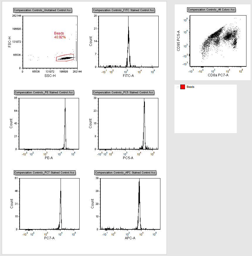
Figure T8.6 Autocomp.fey Layout
In this example, we are setting compensation for all five single-stained controls. However, you can set compensation for as many channels as you like, provided you have a single-stained control for each channel.
3.Click on the Tools tab→Transformations group→Compensation and Unmixing command to open the Compensation and Unmixing navigator (Figure T8.7).
The Compensation and Unmixing navigator can be moved anywhere on the screen; it is dockable and pinnable. Please feel free to move it around the screen or close and reopen as needed while working on this tutorial.
4.Click on the blue plus button, ![]() , to Add a new compensation. A new compensation named New Compensation will be created (Figure below).
, to Add a new compensation. A new compensation named New Compensation will be created (Figure below).
5.Select the New Compensation.
6.In the Automatic Compensation Setup tab, under Step 1 - Select single-stained controls, click on the Add data for compensation button ![]() (Figure T8.7).
(Figure T8.7).
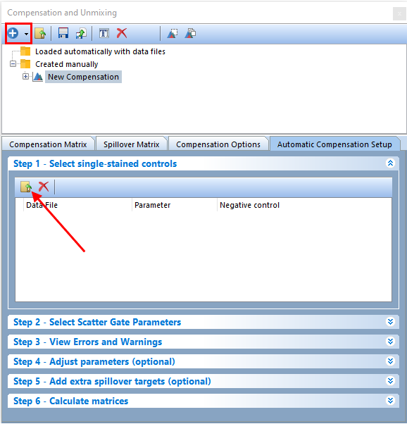
Figure T8.7 Compensation and Unmixing navigator: use to add new compensations, edit definitions, create Automatic Compensations, and unmix spectral signatures
7.The Standard Open Data Dialog will appear (Figure T8.8).
Note: based on your User Options, the Advanced Open Data Dialog may appear. If the Advanced Open Data dialog appears, please select the ![]() button to access the Standard Open Data Dialog.
button to access the Standard Open Data Dialog.
Multiple-select the following six files from the Tutorial Sample Data archive (Figure T8.8):
a.Compensation Controls_APC Stained Control.fcs
b.Compensation Controls_FITC Stained Control.fcs
c.Compensation Controls_PC5 Stained Control.fcs
d.Compensation Controls_PC7 Stained Control.fcs
e.Compensation Controls_PE Stained Control.fcs
f.Compensation Controls_Unstained Control.fcs
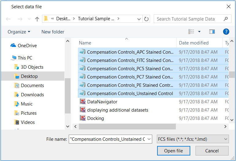
Figure T8.8 - Use the Select Data File window to select all of the files for use in the Automatic Compensation Setup.
8.Click Open file.
Notice all of the single-stained control files and the unstained control file have been brought into the Select single-stained control window and have been assigned the correct parameter and assigned a negative. You may correct the Parameters and define the Negative Control used per control as necessary. When loading a universal negative, or unstained sample, it is assigned automatically as the Negative control for each single-stained control (Figure T8.9).
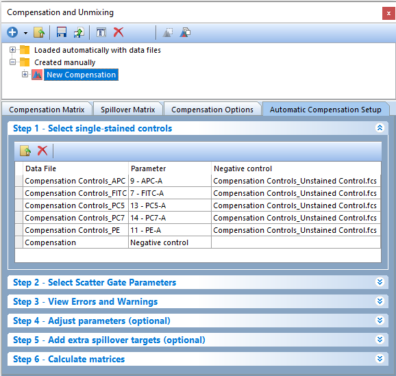
Figure T8.9 Files for controls have been added to Step 1 in the Automatic Compensation Setup and are matched automatically to their respective parameters.
9.FCS Express will automatically create a page for Scatter Plot and also for each individual Single Stained control. Additionally, FCS Express will automatically create pages to accomodate the Spillover Spreading Matrix and the Cross Stain Index Matrix.
Eight new pages will be created (Figure T8.10):
•Scatter Plot
•APC-A
•FITC-A
•PC5-A
•PC7-A
•PE-A
•Spillover Spreading Matrix
•Cross Stain Index Matrix
Figure T8.10 Tabs for new pages created from Step 3
The Scatter Plot page contains a plot based on the parameters selected in Step 2, while the rest of the pages (single-stained control pages) contain a scatter plot and two histograms for each parameter compensated. The top histogram shows the positive population from the single stain control for the parameter, while the bottom histogram shows the negative population from the universal negative control. A histogram marker has been created automatically for each positive and negative population. All of the histogram markers are children of the Scatter Gate, which means adjusting the Scatter Gate will cause the histogram markers to update in real-time.
We now will adjust the Scatter Gate to refine the single-stained and negative populations.
To better appreciate plot adjustments, turn on the Multiple Page view by:
10. Clicking on the View tab→Multiple Page group→Two Pages (Vertical) command.
11. Selecting the Scatter Plot page for the left page.
12. Selecting the FITC-A control page for the right page. Your screen now should resemble Figure T8.11.
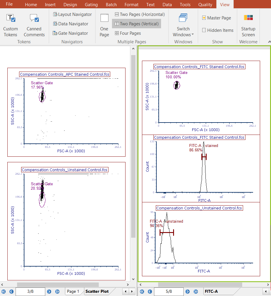
Figure T8.11 Clicking the Build Histograms button results in a Scatter Plot page and a new page for every single-stained control.
13. Click the Gating tab→Create Gates group→Rectangle command.
14. Draw a gate around the beads population on the bottom plot titled "Compensation Controls_Unstained Control" of Scatter Plot page; gate should resemble one on plot in Figure T8.12.
A Create New Gate dialog appears.
15. Chose the Replace an existing gate radio button (Figure T8.12).
16. Choose Scatter Gate from the bottom of the drop-down list (Figure T8.12).
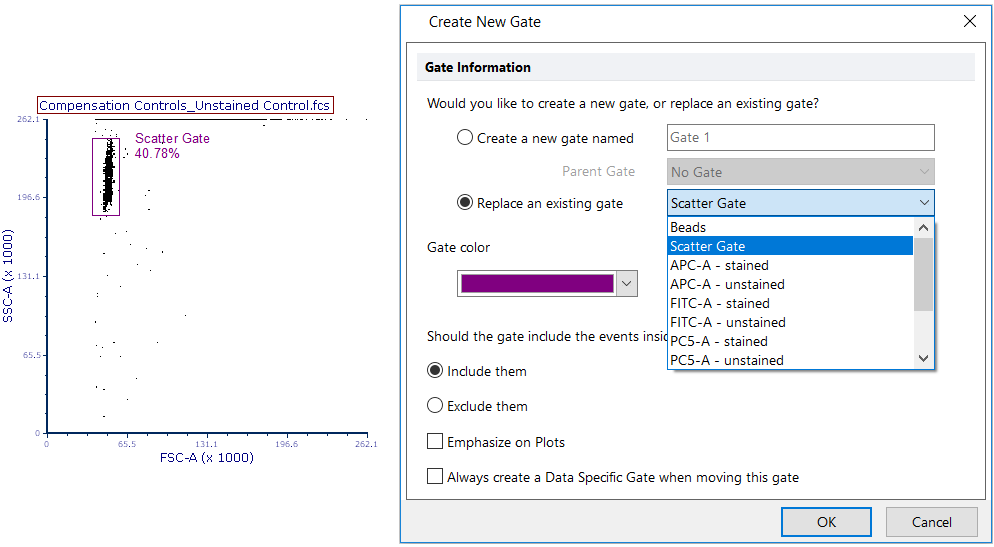
Figure T8.12 Creating a gate around the bead population on the plot and choosing to replace the Scatter Gate with the newly created gate.
17. Click OK.
Notice that the original scatter gate has been replace with the new one you defined. It is convenient to replace the original scatter gate because all the single stained control histograms in the layout are already using that gate. If we had created a new gate, we would have had to apply that new gate to all the single stained control histograms. Notice that the subsequent single stain control histogram pages have updated to use this new gate.
User may also decide to refine markers position in the following pages of the layout (the ones containing single staining control histograms).
18.The Compensation Matrix and the Spillover Matrix will be created after introducing the single stained controls into Step 1.
Description of steps performed automatically by FCS Express that can be adjusted by the user as needed.
Note: Individual steps can be modified manually by the user. Any changes will result in the Compensation Matrix and Spillover Matrix being automatically recalculated.
Step 2 - Select Scatter Gate Parameters (Figure T8.13).
A user can change parameters as preferred by clicking the down arrows to access drop down lists (Figure T8.13). FCS Express will automatically select the X Parameter for Scatter Gate and the Y Parameter for Scatter Gate. A user can modify the auto-selected parameters as needed.
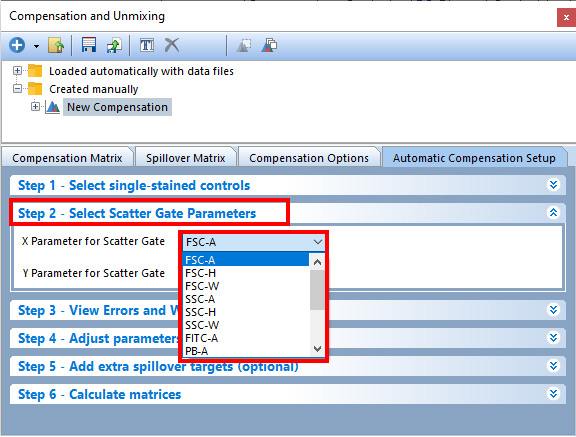
Figure T8.13 Step 2 - Select Scatter Gate Parameters of Automatic Compensation Setup
Step 3 - View Errors and Warnings (T8.14).
Any errors or warnings that prevent histograms being built in Step 1 for the AutoCompensation will be found in this step (T8.14). If there was something wrong with the files or parameters you selected in the previous step, an error message will appear here to let you know what the problem was. If there are no Errors and Warnings the following message will appear - Successfully built histograms for AutoCompensation.
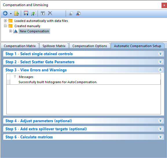
Figure T8.14 The View Errors and Warnings in Step 3 alert the user to any errors that prevented a new page for scatter parameters and a new page containing a positive control and negative control histogram for each individual stain.
Steps 4 and 5 of the Automatic Compensation Setup are optional, and we will them in the next section of this tutorial.
19. Click on Step 6 - Calculate matrices in the Compensations navigator. This step allows the user to determine the statistic to use for calculating the matrices. The Median is selected by default. Making adjustments to the statistic will result in recalculating of the matrices.
| *Note: The checkbox next to Recalculate matrix automatically every time something changes allows FCS Express to modify calculations based on changes made by the user. If this box is not checked, the matrices will not automatically be recalculated and the button Calculate Matrices will need to be used after any changes are made. |
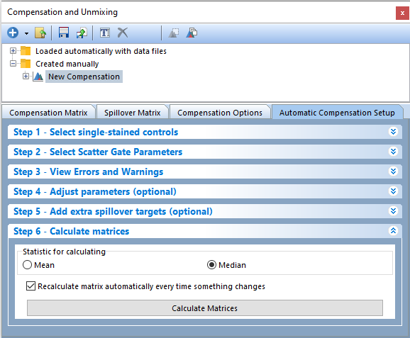
Figure T8.15 Click the Calculate Matrices button to complete your automatic compensation setup.
Then compensation and spillover matrices will be calculated automatically and displayed in the Compensation Matrix and Spillover Matrix tabs of the Compensations navigator. The Editor view (highlighted in red in Figure T8.16 below) can be changed from Matrix Editor to List Editor to view the compensation definitions in matrix or list form. This may also be done in the Spillover Matrix tab.
Note: Your values may differ slightly from figure T8.16 due to differences in how the scatter gate was positioned in steps 15-20 of this tutorial.
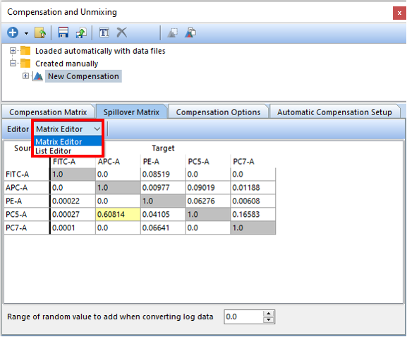
Figure T8.16 The Spillover Matrix created from the Automatic Compensation Setup. The red box indicates you can change from Matrix Editor to List Editor view. The Spillover Matrix tab will display the spillover matrix for your compensation definition.
We will now switch back to a one page view and apply our new automatic compensation to a multicolor control.
20. Click on the View tab→Multiple Page→One Page.
21. Click on the Compensation Samples page tab to move on the first page of the layout (Figure T8.6).
22. Click on the New Compensation compensation in the Compensation and Unmixing navigator to select it (Figure T8.17).
23. Drag and drop (by click and holding the left mouse button) the New Compensation on top of the Compensation Controls_All Colors.fcs plot in the upper right of the layout (see red arrow in Figure 8.17).
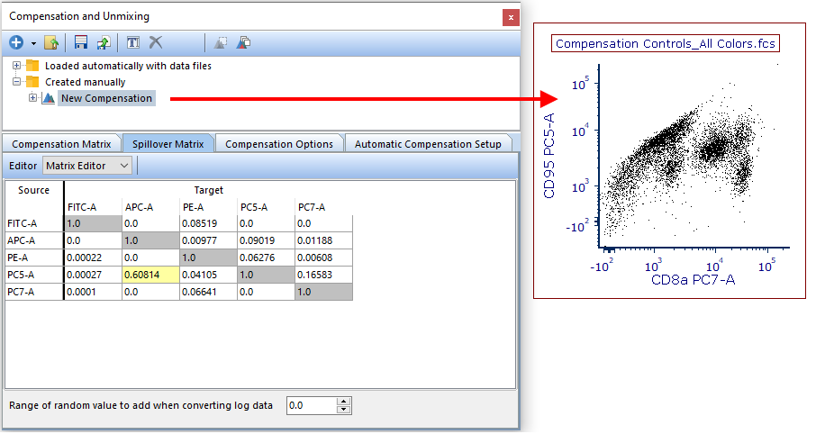
Figure T8.17 Dragging the New Compensation definition from the Compensation and Unmixing navigator and dropping it on a plot will apply that compensation definition to the plot.
The plot will update and show the data properly compensated as in figure T8.18 below.
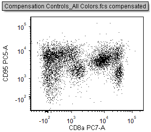
Figure T8.18 The All Colors control plot with the compensation defined in the Automatic Compensation Setup feature applied.
Compensation and Spillover matrices also may be added anywhere in your layout or Microsoft Excel.
24. Click Compensation Matrix within the New Compensation definition to select it (Figure T8.19).
25. Drag the Compensation Matrix to an empty space in the layout and drop it (FigureT8.19).
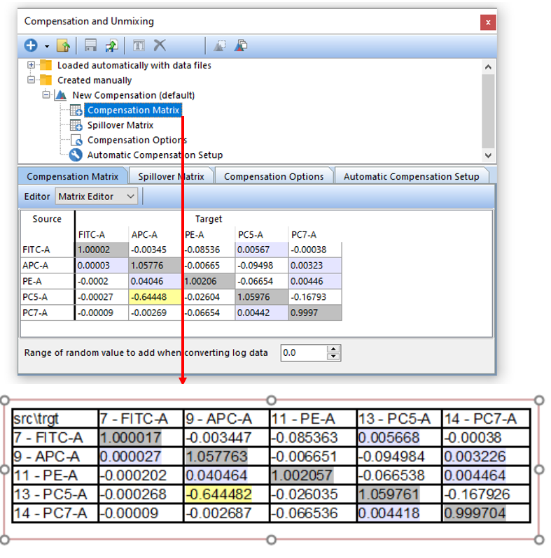
Figure T8.19 Drag and drop the Compensation Matrix to a blank space in the layout (red arrow) to insert a text displaying all of the matrix values.
The compensation matrix now will be displayed in a text box (Figure T8.19). Steps 23 and 24 can be repeated with a drag and drop to Microsoft Excel if you would like the matrices displayed there.
At this point the Automatic Compensation Setup is complete although Step 4 - Adjust parameters (optional) and Step 5 - Add extra spillover targets (optional) may also be used to refine your single stain populations (Adjust parameters) or to have other targets defined without defining a source (Add extra spillover targets). If you would like to learn more about these advanced features please see the tutorials on Automatic Compensation- Optional Steps 4 and 5.
Please see the Creating and Modifying a Compensation Definition chapter of the User Manual for more details about compensation in FCS Express.
