FCS data has traditionally been acquired on either a linear or logarithmic scale, and the appropriate scaling is stored in the header of the FCS data file. Although FCS Express has supported displaying linear data on a logarithmic scale, the data has traditionally been displayed on the same scale as it was acquired.

 

The logarithmic scale has the disadvantage that it cannot display values below zero. This is considered a limitation when performing software compensation where it is common for a significant proportion of compensated data to appear in a "negative" channel. When displayed on a log scale, the negative values are placed on the axis, where they can be easily missed, leading you to overcompensate your data.

 

To overcome this limitation, several additional axis scalings have been developed. These scalings share the general characteristic that they behave linearly close to zero, and behave logarithmically farther away from zero. These scalings also are defined to be able to graph data below zero. Scalings that are a combination of linear and log scalings are called hybrid scalings. More details can be found in the following publications:

 

•Herzenberg LA, Tung J, Moore WA, Herzenberg LA, Parks DR. Interpreting flow cytometry data: a guide for the perplexed. Nat Immunol 2006;7:681-685.

 

•Parks DR, Roederer M, Moore WA. A New "Logicle" Display Method Avoids Deceptive Effects of Logarithmic Scaling for Low Signals and Compensated Data. Cytometry A 2006;69A:541-545.

 

•Bagwell CB. Hyperlog – A Flexible Log-like Transform for Negative, Zero, and Positive Valued Data. Cytometry A 2005;64A:34-42.

 

•Battye FL. A Mathematically Simple Alternative to the Logarithmic Transform for Flow Cytometric Fluorescence Data Displays. Cytometry A 2006;69A:413-414.

 

 

The axis scale for a given plot can be adjusted using the Axis formatting dialog or manual changes to the scale for a given plot parameter may be remembered and applied automatically to all plots in the layout editing your layout options. All data files, regardless of the scale that they were acquired with, can be displayed in any of the scalings supported by FCS Express. The scaling only affects the display of the data, not the statistics.

 

FCS Express supports the following axis scalings:

 

 

Linear

 

This is the standard linear scaling

 

 

Log

 

This is the standard log scaling

 

 

Log with Negative

 

This is a modified log scaling.

         

 

 

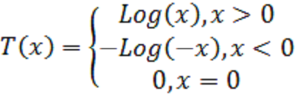
In the normal log function the zero and negative values are undefined, and if they are obtained during compensation they are commonly represented as events stacked on the axis, as is commonly seen in compensated data. In the log with negative function, if negative values are encountered, the log of its absolute value is calculated and displayed on the negative side of the scale, effectively creating a "negative logarithm" display which is a mirror image of its positive counterpart. Zero values are still kept on axis.

 

 

Hyperlog™ – Described in the Bagwell paper, above.

 

The Hyperlog scalings has a coefficient that can be adjusted. The coefficient is called the Transition Point because it describes the transition from the predominantly linear to predominantly log portion of the transform. The transition parameter for the Hyperlog scaling is identical to the b parameter in the Bagwell paper, above.

Transition values are entered in channel units, and do not have to be scaled as described in the Bagwell paper.

Smaller transitions values result in plots which more closely resemble the standard log plots. The precise transition value to use will depend for the most part on your data, and generally a value of at least 30 is required.

 

 

Lin/Log

 

This scale is described in the Battye paper, above.

 

         

 

The Lin/Log has a coefficient that can be adjusted. The coefficient is called the Transition Point because it describes the transition from the predominantly linear to predominantly log portion of the transform. This transform is purely linear below the transition point and purely log above the transition point. The a and c coefficients are matched so that the function is continuous at the transition point.

 

An example of setting the Lin/Log scaling with a Transition Point of 200 is shown in Figure 5.140. Transition values are entered in channel units, and do not have to be scaled as described in the Bagwell paper.

 

 

 

 

Smaller transitions values result in plots which more closely resemble the standard log plots. The precise transition value to use will depend for the most part on your data, and generally a value of at least 30 is required.

 

ArcSinh

 

ArcSinh is an inverse hyperbolic function most widely used with .fcs files generated by CyTOF Mass Cytometry. Unlike standard light based flow cytometry, mass cytometry can produce many true zero signal ("intensity") values. An ArcSinh transformation helps display and visualize values at or near zero with a "spread" as we are accustomed to visualizing with standard flow cytometry data.

ArcSinh values are calculated by dividing the raw intensity value by a cofactor and by then applying the ArcSinh equation to the result of the division (i.e. =Arcsinh(value/cofactor) ). The "cofactor" defines the size of the linear region around 0, with larger cofactors corresponding to a longer linear region. The Arcsinh formula is depicted in Figure 5.141.

 

 

 

 

 

 

Biexponential

 

The biexponential display was popularized by the BD FACSDiva software. As a result of our close collaboration with BD, FCS Express now supports all of the options that FACSDiva does in terms of displaying biexponential data. In fact, we have implemented FACSDiva's proprietary algorithm for calculating the transition point (i.e. Below Zero parameter), so the results from FCS Express will look identical to the results from the FACSDiva software. For more details please refer to the Biexponential Scaling Implementation in FCS Express chapter.

 

When an FCS file that was acquired with BD FACSDiva is opened in FCS Express you will notice that the automatic scaling in FCS Express applies the Biexponential scaling and chooses the Below Zero Parameter (i.e. the transition point) automatically (Figure 5.142).

 

 

 

The Below Zero Parameter can also be manually adjusted by unchecking the Automatic box and selecting the Use the value radio button. The Below Zero Parameter can then be adjusted via the slider bar or by manually entering a value into the text box (Figure 5.143).

 

 

 

The Calculate automatically radio button may also be checked if you would like to change the gate for calculating the display (Figure 5.144, upper pane) or if you would like to change the method for calculation from BD FACSDiva Method to Fifth Percentile (Figure below, lower pane). The Fifth Percentile method automatically set the Below Zero Parameter to the 5th percentile of the negative data of the gate selected in the "With the gate" drop-down menu (Figure below, upper pane).

 

 

 

 

 

 

 

You may also choose to Automatically set the plot's minimum value by checking/unchecking the associated box. When the Automatically set the plot's minimum value is checked the axis minimum is set to optimize the display by not displaying outliers. When unchecked the entire range of data, including outliers, will be displayed.