Automatic Compensation - Optional Steps 3 and 4
To adjust parameters and extra spillover targets:
Once you have completed Step 2 of the Automatic Compensation Setup you may proceed directly to Step 5 to calculate the matrices or you can go through Step3 and/or Step 4. This tutorial will walk you through a sample compensation setup that uses also Step 3 and Step 4. If you are not yet familiar with automatic compensation in FCS Express please complete the Automatic Compensation tutorial before starting this section.
•Step 3 - Adjust parameters (optional) allows you to base your single stained controls on gates other than the default marker gates that were created during the automatic compensation setup.
o Adjust parameters is useful when you would like to refine the populations that are used for calculating compensation. For instance, if the Automatic Compensation Setup does not make a good estimate of the population or if you would like to use a population from another file, gate, gating hierarchy, or plot Step 3 would prove very useful. Parameters may be adjusted or changed all together by dragging and dropping a plot or gate onto the parameter for the Stained and Unstained columns. If a gate is dropped the compensation definition will be based on that gate and plot it originated from (keep in mind any gating hierarchy you have defined with a gate will be used) . If a plot is dropped, the compensation definition will be based on the plot that you just dropped, with the gating being unchanged. Dragging and dropping new plots, files, or gates in this section will allow you to override the automatic setup and use gates and plots of your choice.
• Step 4 - Add extra spillover targets (optional) will allow you to have other fluorescence targets defined without defining a source fluorescence.
oAdding extra spillover targets is useful if you would like to have an idea of what spillover would look like if an extra parameter was added in future experiments. To add an extra spillover target simply check the box for the extra target you would like to add. Note. Extra spillover targets will only appear for parameters that were acquired with the data.
The layout that will be used for this section of the tutorial is AutoCompAdditionalSteps.fey and it can be found in the Tutorial Sample Data archive. In this layout an automatic compensation setup definition (named New Automatic Compensation) has already been created using the standard default setup described in the previous section. The layout contains 4 pages as follows:
•Gating Strategy and Sample page: The Gate View on this page shows the gating strategy that was created automatically by the compensation setup (purple gates) and the one that we would like to use (red and blue gates). The plots are arranged starting from the top left to show how the gating hierarchy has been applied. Follow the green arrows next to each plot to see how the gates have been applied and defined. The plot labeled SAMPLE COMPENSATION has the New Automatic Compensation definition applied to it. The plot off the page to the right is labeled Data for New Compensation Gates and has no compensation applied to it. The Data for New Compensation Gates plot has gates drawn on the PE positive, PerCPCy5-5 positive, and negative populations. These gates will be used later in the tutorial for the adjust parameters steps.
•Scatter Plot page: This page was created by the Automatic Compensation Setup tool and displays the stained and unstained populations used to calculate the compensation matrix.
•CD 62L YG PE-A control page: This page was created by the Automatic Compensation Setup tool and displays the current gate used to calculate the compensation matrix for the PE parameter.
•CD 4 PerCP-Cy5-5-A control page: This page was created by the Automatic Compensation Setup tool and displays the stained and unstained populations used to calculate the compensation matrix for the PerCPCy5-5 parameter.
In the following steps we will:
•Adjust the parameters to define new gates for the single stained and unstained controls.
•Change the gating hierarchy to make the Scatter Gate (defined by the Automatic Compensation Setup) a child of manually defined gates.
•Add an extra spillover target to view the potential spillover of another target.
1. Select File tab→Open (Figure T3.1).
2. Open the layout AutoCompAdditionalSteps.fey found in the Tutorial Sample Data archive (see above for a description of the layout).
3. Click on the Created manually folder→New Automatic Compensation→Automatic Compensation Setup in the Compensations navigator (figure T8.22 red box).
4. Click on the Add data for compensation button, ![]() , in the Automatic Compensation Setup→Step 1 - Select single-stained controls window (Figure T8.7).
, in the Automatic Compensation Setup→Step 1 - Select single-stained controls window (Figure T8.7).
5. Click on the Data List tab (Figure T8.8).
6. Multiple-select the following files in the Data List (Figure T8.8):
•Specimen_001_PE_CD62L.fcs
•Specimen_001_PerCP Cy5-5 CD4.fcs
•Specimen_001_PE_unstained.fcs
7. Chose the parameter for each data file based on the table below:
Data File |
Parameter |
Specimen_001_PE_CD62L.fcs |
9 - YG PE-A |
Specimen_001_PerCP Cy5-5 CD4.fcs |
10 - PerCP-Cy5-5-A |
Specimen_001_PE_unstained.fcs |
Universal Negative |
8.Click on Step 2 - Build histograms to expand the build histograms window (T8.13).
9.Click on the Build Histograms button (T8.13).
10. A window asking for deleting the layout pages and gates previously created opens. Click Yes.
As in the previous tutorial section we will now make some adjustments to the Scatter Gate to refine the automatically marked/gated single stain and negative populations.
In this instance FSC-H vs FSC-A are not the correct parameters for defining scatter so we will replace the Scatter Gate with a more appropriate one.
11. Select the Scatter Plot page and change the X-Axis parameter of the displayed dot plot to SSC-H.
12. Choose the Gating tab→Create Gates→Rectangle.
13. Draw a gate around the cell population like the one in the Figure below (Figure T8.22a, left panel).
14. In the Create New Gate dialog that appears chose the Replace an existing gate radio button and select Scatter Gate from the bottom of the drop down list (Figure T8.22a, right panel).
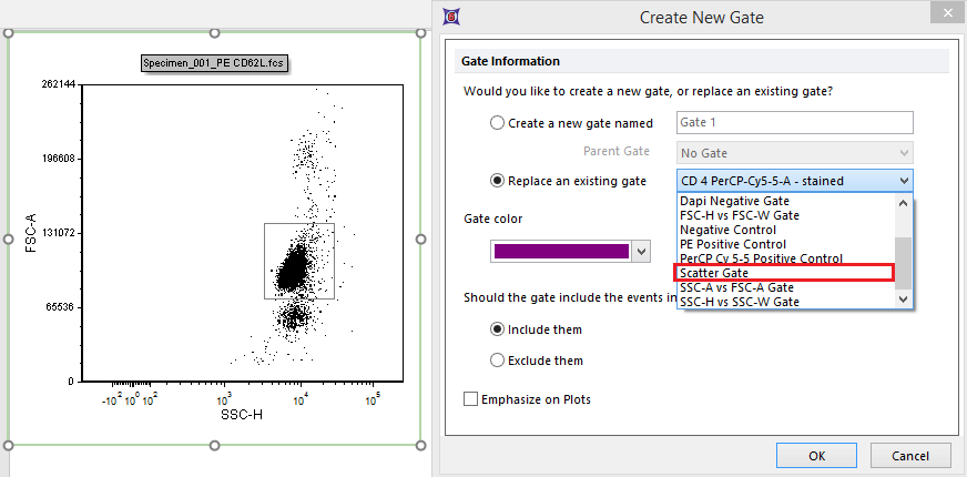
Figure 8.22a - A new Scatter Gate is drawn and used as replacement for the original one.
15. Click OK.
Notice that the original scatter gate has been replace with the new one you defined. It is convenient to replace the original scatter gate because all the single stained control histograms in the layout are already using that gate. If we had created a new gate, we would have had to apply that new gate to all the single stained control histograms. Notice that the subsequent single stain control histogram pages have updated to use this new gate.
User may also decide to refine markers position in the following pages of the layout (the ones containing single staining control histograms).
16. Click on Step 3- Adjust parameters (optional) (figure T8.22b).
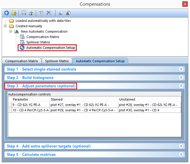
Figure T8.22b - Selecting the Automatic Compensation setup and Step 3 for the New Automatic Compensation definition.
We will now replace the gates that were defined in the Automatic Compensation Setup with gates we have defined manually. These manually defined gates represent the following:
•A gating hierarchy has been defined with all of the FSC and SSC parameters and a Dapi Negative gate. This hierarchy is used to exclude debris and other unwanted events.
•Negative Control Gate: This gate is a child of the Dapi Negative Gate hierarchy. It defines a negative or unstained control population.
•PE Positive Control gate: This gate is a child of the Dapi Negative Gate hierarchy. It defines a PE single color control only population.
•PerCP CY5-5 Positive Control gate: This gate is a child of the Dapi Negative Gate hierarchy. It defines a PerCP CY5-5 single color only population.
17. Click and hold on the Negative Control gate in the gate view (Figure T8.23).
18. Drag the Negative Control gate onto the Unstained column in the CD62L YG PE-A row and drop it here.
19. Click and hold on the Negative Control gate in the gate view.
20. Drag the Negative Control gate onto the Unstained column in the CD4 PerCP-Cy5-5-A row and drop it here.
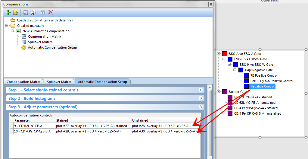
Figure T8.23 - Dragging the Negative Control gate from the gate view to the Unstained column for both parameters.
Now the Step3 - Adjust Parameters (Optional) section should look as in Figure T823b.
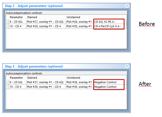
Figure T8.23b The Step3 section after the drag&drop
We previously dragged and dropped the Negative Control gate from the Gate View. We will now use a plot a source for the drag and drop (Figure T8.24).
21. Click and hold on the PE Positive Control gate in the Data for New Compensation Gates plot (off the right hand side of page).
22. Drag and drop it onto the Stained column in the CD62L YG PE-A row and drop it here.
23. Click and hold on the PerCPCY5-5 Positive Control gate in the Data for New Compensation Gates plot (off the right hand side of page) (Figure T8.24).
24. Drag and drop it onto the Stained column in the CD4 PerCP-Cy5-5-A row and drop it here.
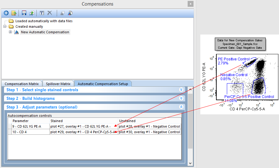
Figure T8.24 - Dragging and dropping gates from a plot to the Stained column in step 3 for each parameter.
Step 3 - Adjust parameters (optional) will look like figure T8.25 below when you are done.
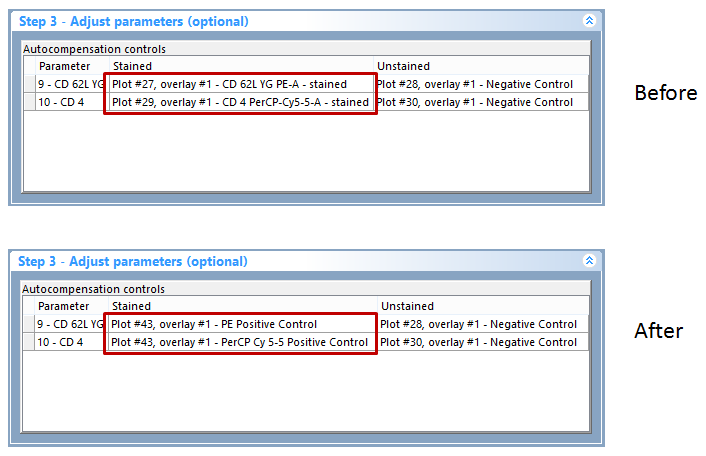
Figure T8.25 - Step 3 - Adjust parameters (optional) after dragging and dropping gates from the gate view and plots onto the stained and unstained population columns.
25. Click now on Step 5 - Calculate matrices.
26. Click the Calculate Matrices button.
Notice that the spillover matrix for the New Automatic Compensation definition has changed (see Figure T8.26 below) to reflect the new gating changes. You can drag and drop any gate or an entire plot to the Stained and Unstained columns in this fashion to customize your Automatic Compensation Setup.
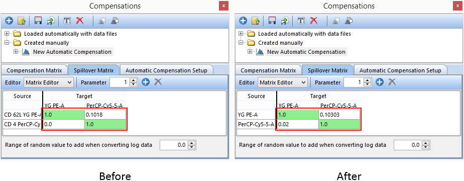
Figure T8.26 - The original Automatic Compensation Setup definition (left) compared to the Automatic Compensation Setup definition (right) that is based on a gating hierarchy and manually defined positive and negative controls.
Another useful trick is to make the Scatter Gate and its children (defined by the Automatic Compensation Setup) children of another gate that you have defined. In the following steps we will make the Scatter Gate a child of the Dapi Negative gate. When the matrix is recalculated the manually entered gating hierarchy for debris exclusion will be taken into account with the Automatic Compensation Setup. We will first close the layout and open it again to reset the changes we have made to the compensations.
27. Select File tab→Close. (Do not save any changes).
28. Select File tab→Open.
29. Open the layout AutoCompAdditionalSteps.fey found in the Tutorial Sample Data archive.
30. Click on the Created manually folder→New Automatic Compensation→Automatic Compensation Setup in the Compensations navigator (figure T8.22 red box).
31. Click on the Add data for compensation button, ![]() , in the Automatic Compensation Setup→Step 1 - Select single-stained controls window (Figure T8.7).
, in the Automatic Compensation Setup→Step 1 - Select single-stained controls window (Figure T8.7).
32. Click on the Data List tab (Figure T8.8).
33. Multiple-select the following files in the Data List (Figure T8.8):
•Specimen_001_PE_CD62L.fcs
•Specimen_001_PerCP Cy5-5 CD4.fcs
•Specimen_001_PE_unstained.fcs Click and hold on the Scatter Gate in the Gate View
33. Chose the parameter for each data file based on the table below:
Data File |
Parameter |
Specimen_001_PE_CD62L.fcs |
9 - YG PE-A |
Specimen_001_PerCP Cy5-5 CD4.fcs |
10 - PerCP-Cy5-5-A |
Specimen_001_PE_unstained.fcs |
Universal Negative |
34. Drag the Scatter Gate on top of the Dapi Negative Gate and drop it here (Figure T8.27).
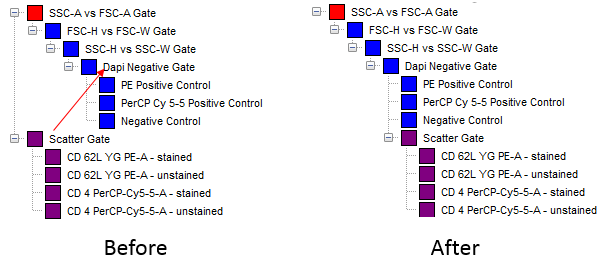
Figure T8.27 - Dragging and dropping the Scatter Gate onto the Dapi Negative Gate to create a new gating hierarchy
Click on Step 5 - Calculate matrices.
35. Click on Step 2 - Build histograms to expand the build histograms window (T8.13).
36. Click on the Build Histograms button (T8.13).
37. A window asking for deleting the layout pages and gates previously created opens. Click Yes.
38. Click the Calculate Matrices button.
Notice that the spillover matrix for the New Automatic Compensation definition has changed (see Figure T8.28 below) to reflect the new gating changes. This is because the plots that were created by the Automatic Compensation Setup were gated on the Scatter Gate so by moving the Scatter Gate in the gating hierarchy the statistics based on these plots were automatically updated.
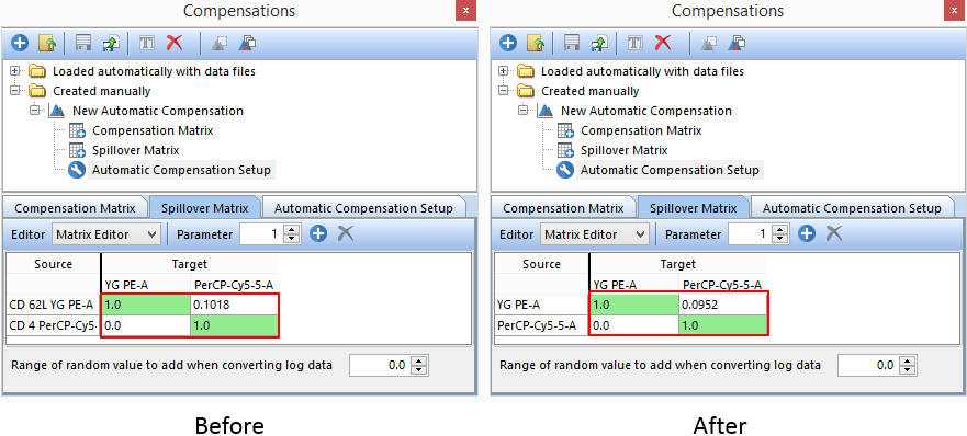
Figure T8.28 - The original Automatic Compensation Setup definition (left) compared to the Automatic Compensation Setup definition (right) that is based on the new gating hierarchy of the Scatter Gate.
We will now use Step 4 - Add extra spillover targets (optional) to determine the theoretical spillover for the FITC parameter.
39. Click on Step 4 - Add extra spillover targets (optional) to expand the window.
40. Check the FITC-A check box (Figure T8.28).
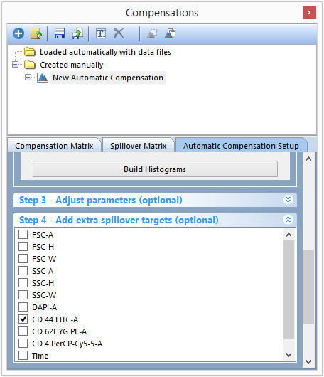
Figure T8.28 - Adding an extra spillover target in Step 4.
41. Click the Calculate Matrices button in Step 5 - Calculate matrices.
The Spillover Matrix tab will now display all of your original parameters along with the FITC-A parameter that you selected in Step 4- Add extra spillover targets (optional) (Figure T8.29). The column for FITC-A in the matrix is displaying the theoretical compensation needed against all other targets.
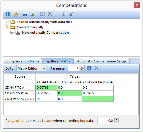
Figure T8.29 - The compensation matrix displaying the extra spillover target that was added. The compensation values for CD 44 FITC-A vs other sources/targets is the theoretical value.
This brings us to the end of the Automatic Compensation Optional Steps 3 and 4 tutorial. Please see the Manual Compensation tutorial or the Compensation section of the manual for more details on compensation in FCS Express.
