Automatically Calculating Compensation Matrices
Instead of manually entering a value to subtract for every target-source pair, or "guessing" the compensation by eye using sliders, FCS Express utilizes a compensation wizard calculate the entire compensation definition for you. For step-by-step instructions on using the Automatic Compensation Setup please see our Automatic Compensation Tutorial. To get started, use the Tools tab→Transformations→Compensation and Unmixing command, open the Compensation and Unmixing window, and add a new compensation with the Add a new compensation button ![]() or you can then click on the Automatic Compensation Setup command (outlined in red below) tab to access the automatic settings (Figure 9.21).
or you can then click on the Automatic Compensation Setup command (outlined in red below) tab to access the automatic settings (Figure 9.21).
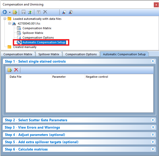
Figure 9.20 The Automatic Compensation Setup tab.
The Automatic Compensation Setup tab contains 6 steps to calculate your compensation. After adding single stained controls in Step 1, individual pages for each compensation control will be created, gates for scatter parameters will be created, and gates for single stained controls will be created. Additional, the compensation matrix will be automatically created. In most cases it is recommended that users review each page and gate automatically created by FCS Express to ensure accuracy of "auto gating" on scatter and control parameters. As changes are made to gates or steps 1 through 6, the compensation matrix will be updated in real time.
Note: Step 4 and step 5 are optional and do not have to be completed to generate a matrix.
•Step 1 - Select single-stained controls (Figure 9.22)
In order to automatically calculate a compensation definition, you will need to provide FCS Express with a positive and a negative population for each parameter you wish to compensate. These population can be provided as:
•an FCS file to use as common (universal) negative control and multiple FCS files to use as single stained positive controls (one for each parameter you wish to compensate)
•a series of single stained control FCS files (one for each parameter you wish to compensate), each containing a negative (self negative) and a positive population
•a mixture of the two above-mentioned scenarios
FCS Express also provides the flexibility for you to choose how to define your positive and negative populations. By default, the main population of interest is defined with gates on 2D Plots (for example, a Scatter Gate on FSC and SSC parameters) while positive and negative populations are automatically defined using markers on histograms (histogram and markers are automatically created for each parameter after adding single stained controls). You will have the option of using an unstained control for each parameter you wish to compensate or use additional user-created gates in Step 4.
1. Click the Add data for auto compensation button, ![]() , to add files that will serve as compensation controls.
, to add files that will serve as compensation controls.
2. Confirm the correct Parameters were automatically matched to the appropriate data file. By default, FCS Express will use the Keyword for Parameter Matching selected in the FCS File Options→Instrument Specific Settings to match the contents of the data file name with the appropriate Parameter. Options for Parameter Matching include the keywords for Name, Stain, Name and Stain, Stain and Name, and Display Name. FCS Express will attempt matching parameters but you may need to review or select the parameters manually via the next step.
3. If any Parameter does not automatically match or is incorrectly matched, you may;
a. Use the Parameter drop down menu to choose the correct parameter for each single stained control or universal negative.
b. Change the data file name to include the desired Parameter Name or Stain Keyword then re-add the data file to Step 1.
4. If a universal Negative Control is selected from the Parameter list in Step 1 (image below), that file will be used by default to define the negative control populations for each parameter.
a.If no universal negative control is selected, you may set each file as its own negative control by selecting the option to use self as negative from the Negative Control drop down menu.
b.You will also have the option to use additional files or populations defined in user-created gates at Step 4 to define positive and negative populations.
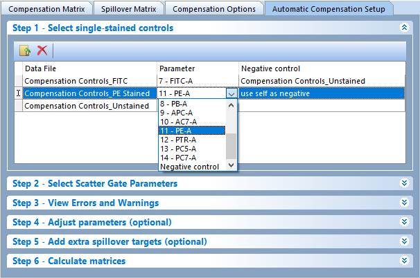
Figure 9.21 Step 1 - Select single-stained controls. Add compensation control data files and choose their respective channels from the Parameter drop down list.
5. If there were no Errors and Warnings highlighted in red (Step 3), the following items will be created: (Figure 9.23):
• Scatter Plot Layout Page: A page will be created with a density plot displaying SSC vs FSC and a Scatter Gate (see Step 2) for the first single-stained control file. If a Universal negative is present, a second density plot will be displayed with the same SSC vs FSC parameters and Scatter Gate for the Universal negative. The Scatter Gate is automatically created and used to define the "live" cells or cells of interest in your compensation controls.
Note: All of the fluorescence gates are children of the Scatter Gate, which means adjusting the Scatter Gate will cause all other gates to update in real time. Step 2 of the automatic compensation workflow allows the user to redefine which parameters FCS Express should use to create the Scatter Gate. Changes made to the parameters (e.g., SSC-H instead of SSC-A) in Step 2 will automatically be updated on the plots created on compensation pages.
The Scatter Gate can be modified by moving the gate, using the replace gate feature or by using Data Specific Gates. To replace the Scatter Gate with a new gate:
• Draw a gate around the population of interest.
• Choose the Replace an existing gate radio button in the Create New Gate dialog.
• Select Scatter Gate from the drop down menu.
• Click OK.
(Note: These steps are also described in the Automatic Compensation Setup tutorial).
•Single Stained Control Layout Pages: A new page will be created for every parameter you are compensating (e.g., "FITC-A control", "APC-A control" in the image below). The page will display one density plot (SSC vs FSC) for the single-stained control for that page and include a Scatter Gate, one histogram with the stained population marked and one histogram with the unstained population marked. Markers will be placed based on FCS Express auto recognition of peaks, but can be adjusted. In addition, each single-stained control's Scatter Gate can be converted to a Data Specific Gate for file-specific adjustment of the gate positions.
Note: the unstained population histogram will only appear if a universal negative is chosen. If a universal negative is not present, only the SSC vs FSC density plot and single histogram with two markers (for positive and negative populations) will appear.
•Spillover Spreading Matrix page: this page depicts a spreadsheet with the Spillover Spreading Matrix values for every pair of dyes included in the compensation matrix.
•Cross Staining Index matrix: this page depicts a spreadsheet with the Cross Stain Index Matrix values for every pair of dyes included in the compensation matrix.
•Gates: New gates will be created for the Scatter Gate and each stained and unstained set up markers will be converted and linked to gates. After the initial "auto-gating" all the gates and markers may be manually adjusted as needed. (Note: A Gate View will not automatically be inserted.)
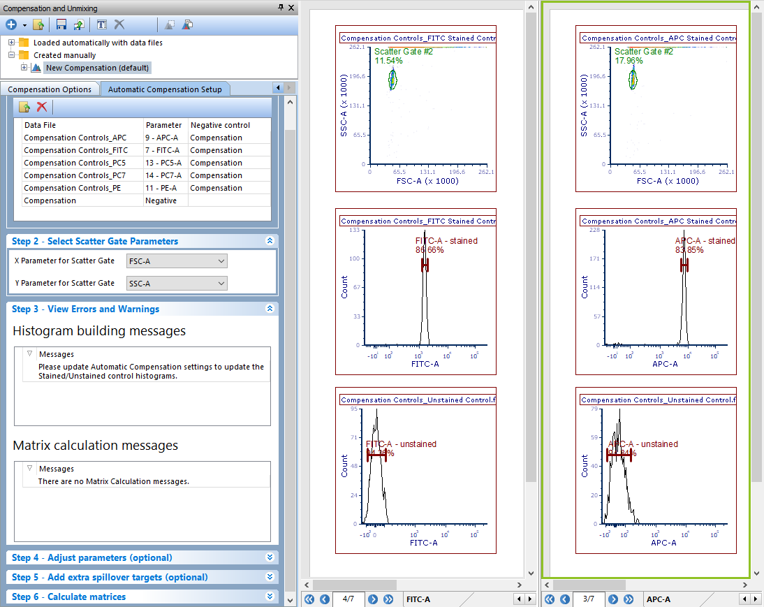
Figure 9.22 Layout after Step 3 of Autocompensation setup. Note the Scatter Plot, FITC control, and APC control pages. Also notice that a density plot for SSC vs FSC has been created with a Scatter Gate automatically applied. Histograms with markers for the stained and unstained populations have also been automatically created.
•Step 2 - Select Scatter Gate Parameters (Figure 9.24)
When building the automatic compensation, FCS Express will automatically create a Scatter Gate to capture your population of interest (eg. stained cells or beads). By default, the Scatter Gate is created using the first available FSC and SSC parameters. If these parameters are not appropriate for your Scatter Gate, or you would like to change the parameters used to create the Scatter Gate, you can define the parameters FCS Express uses to create the Scatter Gate on Step 2 - Select Scatter Gate Parameters.
Adjustments made to the X and Y parameters will automatically be updated on the axes of the plots present on the layout pages created for compensation.
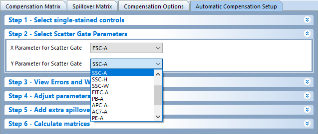
Figure 9.23 Step 2 - Select Scatter Gate Parameters. Choose the respective X and Y Scatter Gate parameters from the dropdown menu.
•Step 3: View Errors and Warnings (Figure 9.25)
•If FCS Express finds problems with either the files or parameters you selected in the previous steps, or in the matrix calculation, warning/error messages will appear in the Histogram building messages and/or in the Matrix calculation messages sections of Step 3 respectively.
To let the user know that FCS Express found issues, Step 3 will be highlighted accordingly: yellow indicates when Warnings are present, and red when Errors are present.
If there are no errors found, the following message will appear - Successfully built histograms for AutoCompensation.
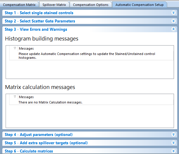
Figure 9.24 Step 3: View Errors and Warnings.
In the example below, the PE control was added twice to the file list. Step 3 is colored red and an the error appears in the Histogram building messages section (Figure 9.26)
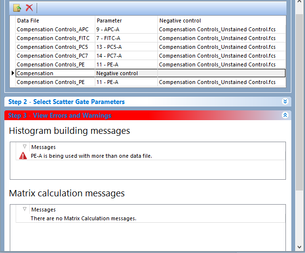
Figure 9.25 Step 3: View Errors and Warnings displaying a warning for duplicated parameter.
In the example below, the marker defining the "APC-A stained" population was improperly placed causing the number of event in that population being zero. As a result, Step 3 is colored red and an error appears in the Matrix calculation messages section (Figure 9.27)
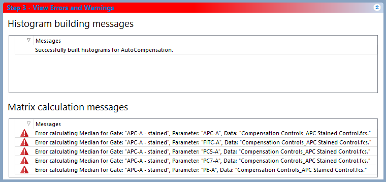
Figure 9.26 Step 3 displaying an error in the "Matrix calcualtion messages" section.
Step 4 - Adjust parameters (optional) (Figure 9.28) is useful when you would like to refine the populations that are used for calculating compensation. Dragging and dropping new plots, files, or gates in this section will allow you to override the automatic setup and use gates and plots of your choice. For instance, if the Automatic Compensation Setup does not make a good estimate of the population or if you would like to use a population from another file, gate, or plot, Step 4 would be useful. Parameters may be adjusted or changed altogether by dragging and dropping a plot or gate onto the parameter for the Stained and Unstained columns. If a gate is dropped, the compensation definition will be based on that gate, including its hierarchical position visible in the Gate View object. If a plot is dropped, the compensation definition will be based on the entire population on the plot.
Note: If you have adjusted a parameter, the compensation matrix will automatically be recalculated.
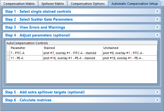
Figure 9.27 The Adjust parameters dialog displaying the currently defined parameters, plots, and gates.
Instructions for adjusting parameters (Figure 9.29):
1.Click and hold on a gate or plot.
2.Drag the gate or plot to appropriate cell in the Auto-compensation controls table (red arrow).
3.Release the mouse button.
The new gate and or plot will appear by name in the appropriate cell in the Auto-compensation controls table of the Adjust parameters pane (Figure 9 below, green arrow).
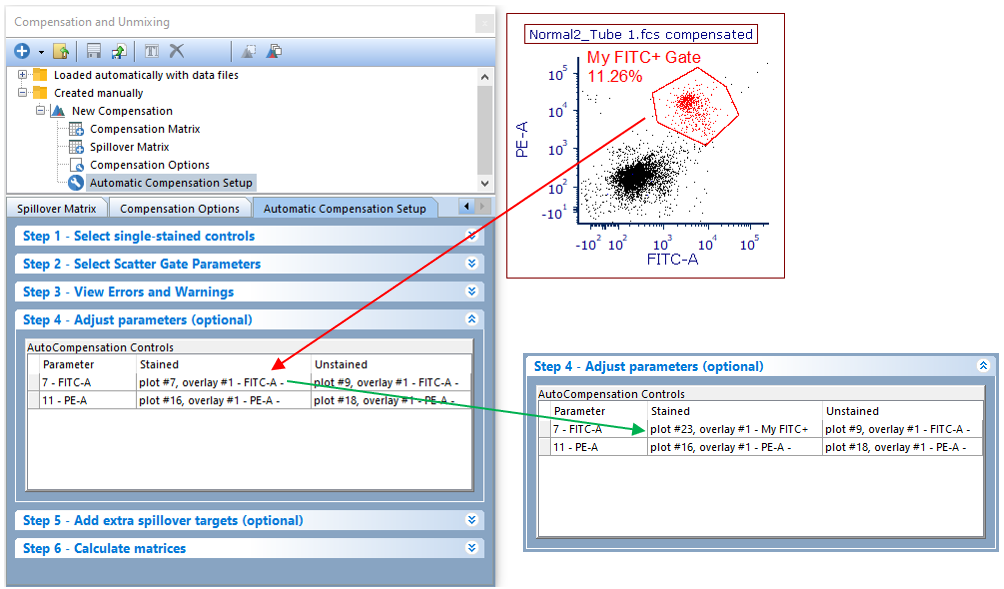
Figure 9.28 To change a parameter plot or gate drag the gate or plot onto the plot you wish to change. The plot information will then update to the newly choosen gate or plot.
•Step 5: Add extra spillover targets (optional) (Figure 9.30)
Adding extra spillover targets allows you to have other targets defined without defining a source. This is useful if you would like to have an idea of what spillover would look like if an extra parameter was added in future experiments. To add an extra spillover target simply check the box for the extra target you would like to add. Note: extra spillover targets will only appear for parameters that were acquired with the data.
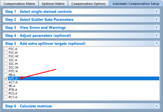
Figure 9.29 The Add extra spillover targets (optional) dialog. Checking a box will calculate the spillover for targets that have no source.
•Step 6: Calculate matrices (Figure 9.31)
In step 6 the user may choose to Calculate Matrices based on the Mean or Median depending on your preference for your data and experiment. Click on the radio button for either choice to apply your preference. The initial matrices are calculated by utilizing the Median by default and will be update automatically if Mean is selected.
By default, FCS Express will automatically calculate and recalculate the matrix as changes are made to gates or other settings giving users "real time" feedback on adjustments to gates. If you would like to manually choose when to calculate the matrix, uncheck the Recalculate matrix automatically ever time something changes box and press the Calculate Matrices button.

Figure 9.30 Step 6 of the Automatic Compensation Setup wizard.
The Spillover Matrix or Compensation Matrix can be viewed in the Compensations and Unmixing window by clicking on the appropriate tab in the navigator. See the Spillover Matrix displayed below. (Figure 9.32). You may edit any of the source-target pairs through the Compensation Matrix, Spillover Matrix, or make new adjustments in the Automatic Compensation Setup. In the Compensation Options tab, you can set how the new compensated parameters are displayed in the parameter list and whether to retain or overwrite the original uncompensated parameters.
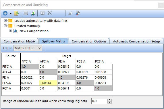
Figure 9.31 The Compensation Matrix after the Automatic Compensation Setup is complete.
The automatic compensation setup settings are saved with the layout. To create another compensation matrix from a different set of data, simply add a new compensation with the Create a new compensation button ![]() and begin the Auto compensation setup process again.
and begin the Auto compensation setup process again.
We also suggest that you use the compensation determined in the Automatic Compensation Setup and apply it to different layouts and files rather than re-creating the same compensation definition many times.
A step-by-step description of the Automatic Compensation Setup feature is provided in our tutorials at Compensation Tutorial.
