Pre-Defined Algorithms

Contents
Pre-Defined Algorithms are a group/folder of pipeline steps which contain the individual components for running an algorithm. For instance, you may choose SPADE or tSNE as a standard transformation from the Add Transformation button, but if you would like to fine tune individual components of the algorithm, or add additional pipeline steps of your own design, using a pre-defined step will allow you additional flexibility and granularity.
The table below describes the pre-defined Algorithm pipeline steps that are available in FCS Express. If you would like to recommend additional Pre-Defined Algorithms to be provided with FCS Express, please contact support@denovosoftware.com.
Algorithm Name
|
Description |
|---|---|
|
FlowAI allows the user to perform quality control on flow cytometry data in order to improve both manual and automated downstream analysis.
The algorithm removes events with anomalous values by taking into account three aspects of a flow cytometry data file: 1. Flow rate 2. Signal acquisition 3. Dynamic range
In FCS Express, the FlowAI pre-defined algorithm step automatically creates a Pipeline Folder that includes the steps listed below, allowing users to easily create a pipeline to run FlowAI on the selected input parameters and/or population/gate selected in the main pipeline body.
Important Notes:
1. FlowAI (and more specifically the Signal Acquisition and the Dynamic Range Downsampling steps) is intended to be run on Linearly scaled data. If one or multiple Scaling steps are present in the pipeline upstream of the FlowAI step, please be sure to select linearly scaled parameters (e.g. unscaled parameters) as input parameters for both the Signal Acquisition Downsampling and the Dynamic Range Downsampling steps.
2. FlowAI (and more specifically the Signal Acquisition and the Dynamic Range Downsampling steps) is intended to be run on non-compensated data. By default, FCS Express applies the compensation matrix associated with the data file (or the default compensation) every time a file is loaded into the layout. By default, FCS Express does not display the non-compensated parameters since usually they are not of interest as plots can easily be displayed with or without compensation as needed. Because FlowAI requires non-compensated data parameters, the following steps should be preformed ahead of using FlowAI:
i.Change the New Compensated Parameters Should setting in the Layout Options so that compensated parameters will be appended to the data file as new parameters. That change will allow both compensated and non-compensated parameters to be accessible when a file is loaded. ii.In the pipeline root step, use the Select Template from Selected Plot option to select a template dataset from a plot existing in the layout. That will allow both compensated and non-compensated parameters to be accessible when the data is used the pipeline. iii.Be sure to select non-compensated parameters as input parameters for both the Signal Acquisition Downsampling and the Dynamic Range Downsampling steps.
3. Non-compensated parameters can be removed after the FlowAI step if not needed in subsequent steps of the pipeline.
4. Pipeline steps downstream from the FlowAI step can subsequently use scaled and/or compensated data.
For more details on the three specific quality controls performed by FlowAI, please refer to the links below:
•Signal Acquisition Downsampling
For more details on the FlowAI algorithm in general, please refer to the original publication (G. Monaco et al, flowAI: automatic and interactive anomaly discerning tools for flow cytometry data, Bioinformatics, Volume 32, Issue 16, 2016)
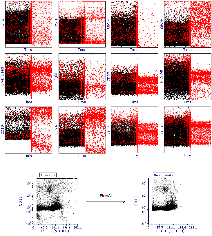
The images provided below are an example dataset cleaned with FlowAI. All parameters (y-axis) have been plotted against Time (x-axis) and events having anomalous values identified by FlowAI have been highlighted in red.
In the bottom panel, a representative plot of the whole dataset has been created using all events (i.e. before the FlowAI cleaning) alongside a plot that displays remaining events after the FlowAI cleaning (Good Events).
|
|
FlowCut allows the user to perform quality control on flow cytometry data in order to improve both manual and automated downstream analysis.
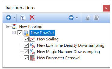
The FlowCut pre-defined algorithm is a four step process. First, a Scaling step is run to scale the data, which is required for FlowCut to proceed. Select all of the fluorescence parameters in this step of the transformation and type in a suffix for the transformed parameters. To perform the second step FlowCut removes acquisition regions with fewer events and then cleans the remaining data based on multiple quality control tests. To perform the third step, FlowCut separates events along the time axis into equally sized segments (parameter defaults to 500 events in FCS Express) and calculates if any of the segments should be removed because they are statistically different than the others. The fourth step (i.e. Parameter Removal), allows to remove any unneeded parameters the data.
In FCS Express, the FlowCut pre-defined algorithm automatically creates a Pipeline Folder that includes the four steps above, allowing users to easily run FlowCut on the desired input parameters and events. •Low Time Density Downsampling
|
|
FlowSOM is a clustering and visualization tool that facilitate the analysis of high-dimensional data. FlowSOM clusters the input dataset using a Self-Organizing Map allowing users to cluster large multi-dimensional data sets in a short time.
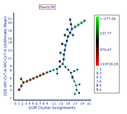
The resulting clusters are then presented to the user as a Minimum Spanning Tree in which each clusters (depicted as a node of the tree) are connected to the closest (i.e. more similar in term of position in the multidimensional space) cluster.
FlowSOM also performs a second clustering step (called meta-clustering) in which clusters, not events, are clustered together based on their similarity. Meta-clustering is a very useful step to group similar clusters together and find meta-clusters which better represent the biological populations in the dataset. The meta-clustering step is performed by running the Consensus Clustering pipeline step in FCS Express.
For more details on FlowSOM algorithm, please refer to the original article publish by Sofie Van Gassen and colleagues: FlowSOM: Using Self-Organizing Maps for Visualization and Interpretation of Cytometry Data; Sofie Van Gassen et al, Cytometry Part A, 2015.
The FlowSOM pre-defined algorithm step automatically creates a Pipeline Folder with the following steps listed below, allowing the user to easily run FlowSOM on the selected input parameters and/or population/gate selected in the main pipeline body and allowing additional flexibility to create supporting pipeline steps as needed. Please refer to the links below for additional information on each step.
1.Scaling (this step might not be required, and can be deselected/removed, if the input parameters from FlowSOM have been scaled with another Scaling step upstream FlowSOM) 6.Parameter Removal (this is optional and is intended to remove parameters that are not required downstream FlowSOM, making the parameter list shorter and easier to handle)
Below is an example of FlowSOM tree. Note the meta-clusters (6 in this example) are depicted as colored halos around the nodes. Those sharing the same color belong to the same meta-cluster.
Once the FlowSOM tree is displayed, the Heat Map may be formatted to: •Have well size dependent on a statistic such as number of events in the node •Set the Parameter and Statistic for display •Change the Color Level and Color Scheme •Create gate(s) to identify node(s) of interest, and edit other features
|
|
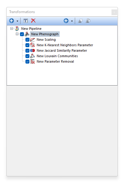
Phenograph is a clustering tool that facilitates the analysis of high-dimensional data. Phenograph first represents the high-dimensional data set with a graph structure. In this representation, each cell is represented as a node and is connected to its neighbors (i.e. the cells most similar to it) via an edge whose weight is set by the similarity between cells. Dense regions of cells will manifest as highly interconnected (i.e. high-density of edges) modules in this graph. Once constructed, the graph is partitioned into subsets of densely interconnected modules, called communities, which represent distinct phenotypic subpopulations.
The Phenograph process is performed through the following steps: •K-Nearest Neighbors Parameter.
For more details on the Phenograph algorithm, please refer to the original publication (J. Levine et al, Data-Driven Phenotypic Dissection of AML Reveals Progenitor-like Cells that Correlate with Prognosis, Cell, 2015 Jul 2;162(1):184-97. doi: 10.1016/j.cell.2015.05.047. Epub 2015 Jun 18)
The output of Phenograph is a cluster assignment parameter called "Louvain Communities" that may be plotted on Histograms, 2D plots and Plate Heat Maps. We suggest using Plate Heat Maps, since they allow users to utilize the following features and visualizations:
•Have well size dependent on a statistic such as number of events in the node •Set the Parameter and Statistic for display •Change the Color Level and Color Scheme •Create Well gates to select one or more clusters (i.e. wells) and use those gates/clusters for downstream analysis.
|
|
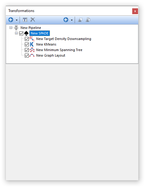
The SPADE pre-defined algorithm step automatically creates a Pipeline Folder with the following steps listed below, allowing users to easily create a pipeline to run SPADE on the input parameters and the input population, and allowing additional flexibility to create supporting pipeline steps as needed.
Please refer to the links below for additional information on each step.
2.Kmeans
Once the SPADE tree is displayed on an Heat Map, the following actions can be performed on the Heat Map: •Have well size dependent on a statistic such as number of events in the node •Set the Parameter and Statistic for display •Change the Color Level and Color Scheme •Create Well gates to select one or more clusters (i.e. wells) and use those gates/clusters for downstream analysis.
For more details on SPADE algorithm, please refer to the SPADE chapter.
|